Have you ever stood outside when it has been snowing and noticed that it feels “quieter” than normal? Have you ever heard your sibling or housemate play music or talk in the room next to you and hear only the lower frequency content on the other side of the wall? People are better at perceptually understanding acoustics than we give ourselves credit for. In fact our hearing and our ability to perceive where a sound is coming from is important to our survival because we need to be able to tell if danger is approaching. Without necessarily thinking about it, we get a lot of information about the world around us through localization cues gathered from the time offsets between direct and reflected sounds arriving at our ears that our brain performs quick analysis on compared to our visual cues.
Enter the entire world of psychoacoustics
Whenever I walk into a music venue during a morning walk-through, I try to bring my attention to the space around me: What am I hearing? How am I hearing it? How does that compare to the visual data I’m gathering about my surroundings? This clandestine, subjective information gathering is important to reality check the data collected during the formal, objective measurement processes of systems tunings. People spend entire lifetimes researching the field of acoustics, so instead of trying to give a “crash course” in acoustics, we are going to talk about some concepts to get you interested in the behavior that you have already been spending your whole life learning from an experiential perspective without realizing it. I hope that by the end of reading this you will realize that the interactions of signals in the audible human hearing range are complex because the perspective changes depending on the relationships of frequency, wavelength, and phase between the signals.
The Magnitudes of Wavelength
Before we head down this rabbit hole, I want to point out one of the biggest “Eureka!” moments I had in my audio education was when I truly understood what Jean-Baptiste Fourier discovered in 1807 [1] regarding the nature of complex waveforms. Jean-Baptiste Fourier discovered that a complex waveform can be “broken down” into its many component waves that when recombined create the original complex waveform. For example, this means that a complex waveform, say the sound of a human singing, can be broken down into the many composite sine waves that add together to create the complex original waveform of the singer. I like to conceptualize the behavior of sound under the philosophical framework of Fourier’s discoveries. Instead of being overwhelmed by the complexities as you go further down the rabbit hole, I like to think that the more that I learn, the more the complex waveform gets broken into its component sine waves.
Conceptualizing sound field behavior is frequency-dependent
One of the most fundamental quandaries about analyzing the behavior of sound propagation is due to the fact that the wavelengths that we work with in the audible frequency range vary in orders of magnitude. We generally understand the audible frequency range of human hearing to be 20 cycles per second (Hertz) -20,000 cycles per second (20 kilohertz), which varies with age and other factors such as hearing damage. Now recall the basic formula for determining wavelength at a given frequency:

Wavelength (in feet or meters) = speed of sound (feet or meters) / frequency (Hertz) **must use same units for wavelength and speed of sound i.e. meters and meters per second**
So let’s look at some numbers here given specific parameters of the speed of sound since we know that the speed of sound varies due to factors such as altitude, temperature, and humidity. The speed of sound at “average sea level”, which is roughly 1 atmosphere or 101.3 kiloPascals [2]), at 68 degrees Fahrenheit (20 degrees Celsius), and at 0% humidity is approximately 343 meters per second or approximately 1,125 feet per second [3]. There is a great calculator online at sengpielaudio.com if you don’t want to have to manually calculate this [3]. So if we use the formula above to calculate the wavelength for 20 Hz and 20kHz with this value for the speed of sound we get (we will use Imperial units because I live in the United States):
Wavelength of 20 Hz= 1,125 ft/s / 20 Hz = 56.25 feet
Wavelength of 20 kHz or 20,000 Hertz = 1,125 ft/s / 20,000 Hz = 0.0563 feet or 0.675 inches
This means that we are dealing with wavelengths that range from roughly the size of a penny to the size of a building. We see this in a different way as we move up in octaves along the audible range from 20 Hz to 20 kHz because as we increase frequency, the number of frequencies per octave band increases logarithmically.
32 Hz-63 Hz
63-125 Hz
125-250 Hz
250-500 Hz
500-1000 Hz
1000-2000 Hz
2000-4000 Hz
4000-8000 Hz
8000-16000 Hz
Look familiar??
Unfortunately, what this ends up meaning to us sound engineers is that there is no “catch-all” way of modeling the behavior of sound that can be applied to the entire audible frequency spectrum. It means that the size of objects and surfaces obstructing or interacting with sound may or may not create issues depending on its size in relation to the frequency under scrutiny.
For example, take the practice of placing a measurement mic on top of a flat board to gather what is known as a “ground plane” measurement. For example, placing the mic on top of a board, and putting the board on top of seats in a theater. This is a tactic I use primarily in highly reflective room environments to take measurements of a loudspeaker system in order to observe the system behavior without the degradation from the reflections in the room. Usually, because I don’t have control over changing the acoustics of the room itself (see using in-house, pre-installed PAs in a venue). The caveat to this method is that if you use a board, the board has to be at least a wavelength at the lowest frequency of interest. So if you have a 4ft x 4 ft board for your ground plane, the measurements are really only helpful from roughly 280 Hz and above (solve for : 1,125 ft/s / 4 ft ~280 Hz given the assumption of the speed of sound discussed earlier). Below that frequency, the wavelengths of the signal under test will be larger in relation to the board so the benefits of the ground plane do not apply. The other option to extend the usable range of the ground plane measurement is to place the mic on the ground (like in an arena) so that the floor becomes an extension of the boundary itself.
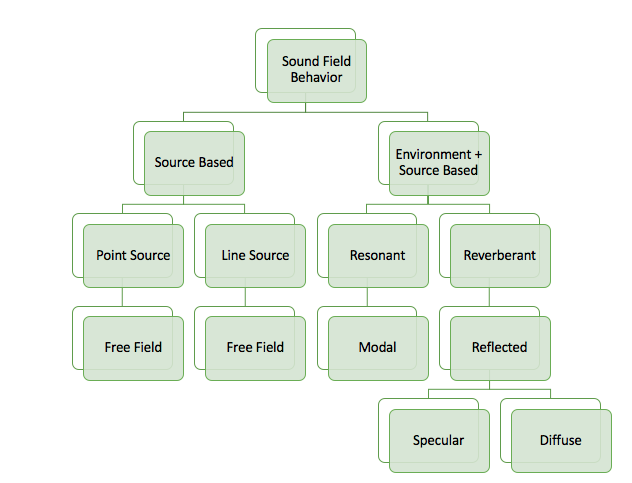
Free Field vs. Reverberant Field:
When we start talking about the behavior of sound, it’s very important to make the distinction about what type of sound field behavior we are observing, modeling, and/or analyzing. If that isn’t confusing enough, depending on the scenario, the sound field behavior will change depending on what frequency range is under scrutiny. Most loudspeaker prediction software works by using calculations based on measurements of the loudspeaker in the free field. To conceptualize how sound operates in the free field, imagine a single, point-source loudspeaker floating high above the ground, outside, and with no obstructions insight. Based on the directivity index of the loudspeaker, the sound intensity will propagate outward from the origin according to the inverse square law. We must remember that the directivity index is frequency-dependent, which means that we must look at this behavior as frequency-dependent. As a refresher, this spherical radiation of sound intensity from the point source results in 6dB loss per doubling of distance. As seen in Figure A, sound intensity propagating at radius “r” will increase by a factor of r^2 since we are in the free field and sound pressure radiates omnidirectionally as a sphere outward from the origin.
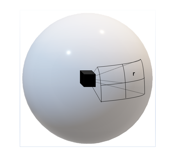
Figure A. A point source in the free field exhibits spherical behavior according to the inverse square law where sound intensity is lost 6dB per doubling of distance
The inverse square law applies to point-source behavior in the free field, yet things grow more complex when we start talking about line sources and Fresnel zones. The relationship between point source and line source behavior changes whether we are observing the source in the near field or far field since a directional source becomes a point source if observed in the far-field. Line source behavior is a subject that can have an entire blog or book on its own, so for the sake of brevity, I will redirect you to the Audio Engineering Society white papers on the subject such as the 2003 white paper on “Wavefront Sculpture Technology” by Christian Heil, Marcel Urban, and Paul Bauman [4].
Free field behavior, by definition, does not take into account the acoustical properties of the venue that the speakers exist in. Free field conditions exist pretty much only outdoors in an open area. The free field does, however, make speaker interactions easier to predict especially when we have known direct (on-axis) and off-axis measurements comprising the loudspeakers’ polar data. Since loudspeakers manufacturers have this high-resolution polar data of their speakers, they can predict how elements will interact with one another in the free field. The only problem is that anyone who has ever been inside a venue with a PA system knows that we aren’t just listening to the direct field of the loudspeakers even when we have great audience coverage of a system. We also listen to the energy returned from the room in the reverberant field.
As mentioned in the introduction to this blog, our hearing allows us to gather information about the environment that we are in. Sound radiates in all directions, but it has directivity relative to the frequency range being considered and the dispersion pattern of the source. Now if we take that imaginary point source loudspeaker from our earlier example and listen to it in a small room, we will hear not only the direct sound coming from the loudspeaker to our ears, but also the reflections from the loudspeaker bouncing off the walls and then back at our ears delayed by some offset in time. Direct sound often correlates to something we see visually like hearing the on-axis, direct signal from a loudspeaker. Since reflections result from the sound bouncing off other surfaces then arriving at our ears, what they don’t contribute to the direct field, they add to the reverberant field that helps us perceive spatial information about the room we are in.
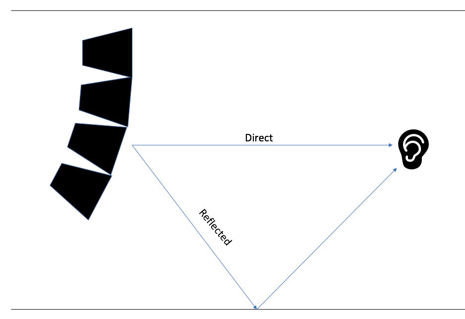
Signals arriving on an obstructed path to our ears we perceive as direct arrivals, whereas signals bouncing off a surface and arriving with some offset in time are reflections
Our ears are like little microphones that send aural information to our brain. Our ears vary from person to person in size, shape, and the distance between them. This gives everyone their own unique time and level offsets based on the geometry between their ears which create our own individual head-related transfer functions (HRTF). Our brain combines the data of the direct and reflected signals to discern where the sound is coming from. The time offsets between a reflected signal and the direct arrival determine whether our brain will perceive the signals as coming from one source or two distinct sources. This is known as the precedence effect or Haas effect. Sound System Engineering by Don Davis, Eugene Patronis, Jr., & Pat Brown (2013), notes that our brain integrates early reflections arriving within “35-50 ms” from the direct arrival as a single source. Once again, we must remember that this is an approximate value for time since actual timing will be frequency-dependent. Late reflections that arrive later than 50ms do not get integrated with the direct arrival and instead are perceived as two separate sources [5]. When two signals have a large enough time offset between them, we start to perceive the two separate sources as echoes. Specular reflections can be particularly obnoxious because they arrive at our ears either with an increased level or angle of incidence such that they can interfere with our perception of localized sources.
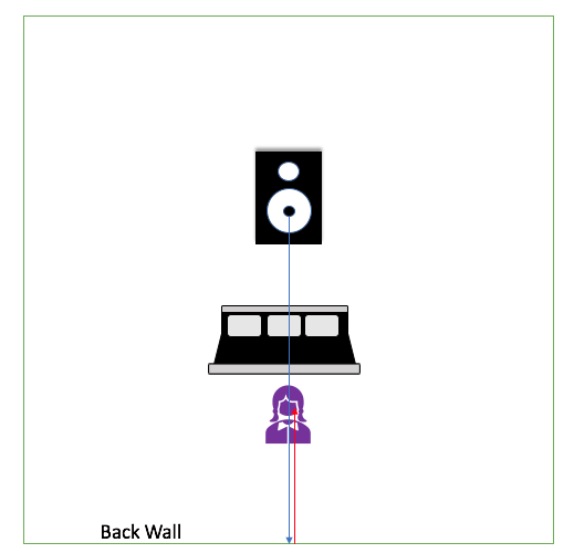
Specular reflections act like reflections off a mirror bouncing back at the listener
Diffuse reflections, on the other hand, tend to lack localization and add more to the perception of “spaciousness” of the room, yet depending on frequency and level can still degrade intelligibility. Whether the presence of certain reflections will degrade or add to the original source are highly dependent on their relationship to the dimensions of the room.
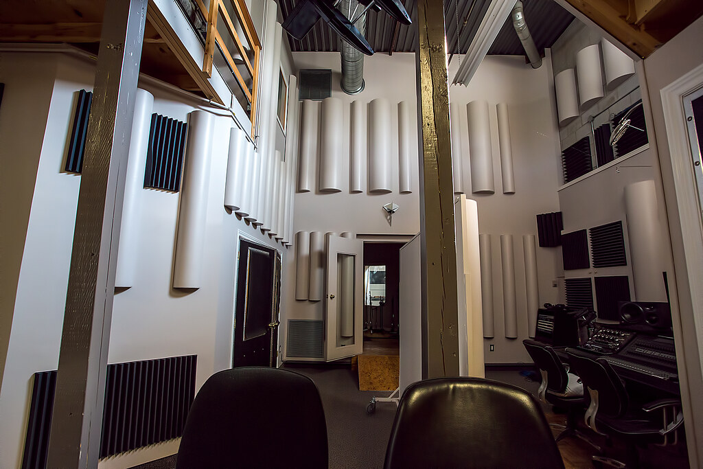
Various acoustic diffusers and absorbers used to spread out reflections [6]
In the Master Handbook of Acoustics by F. Alton Everest and Ken C. Pohlmann (2015), they illustrate how “the behavior of sound is greatly affected by the wavelength of the sound in comparison to the size of objects encountered” [7]. Everest & Pohlmann describe how the varying size of wavelength depending on frequency means that how we model sound behavior will vary in relation to the room dimensions. There is a frequency range at which in smaller rooms, the dimensions of the room are shorter than the wavelength such that the room cannot contribute boosts due to resonance effects [7]. Everest & Pohlmann note that when the wavelength becomes comparable to room dimensions, we enter modal behavior. At the top of this range marks the “cutoff frequency” to which we can begin to describe the interactions using “wave acoustics”, and as we progress into the higher frequencies of the audible range we can model these short-wavelength interactions using ray behavior. One can find the equations for estimating these ranges based on room length, width, and height dimensions in the Master Handbook of Acoustics. It’s important to note that while we haven’t explicitly discussed phase, its importance is implied since it is a necessary component to understanding the relationship between signals. After all, the phase relationship between two copies of the same signal will determine whether their interaction will result in constructive or destructive interference. What Everest & Pohlmann are getting at is that how we model and predict sound field behavior will change based on wavelength, frequency, and room dimensions. It’s not as easy as applying one set of rules to the entire audible spectrum.
Just the Beginning
So we haven’t even begun to talk about the effects of properties of surfaces such absorption coefficients and RT60 times, and yet we already see the increasing complexity of the interactions between signals based on the fact we are dealing with wavelengths that differ in orders of magnitude. In order to simplify predictions, most loudspeaker prediction software uses measurements gathered in the free field. Although acoustic simulation software, such as EASE, exists that allows the user to factor in properties of the surfaces, often we don’t know the information that is needed to account for things such as absorption coefficients of a material unless someone gets paid to go and take those measurements. Or the acoustician involved with the design has well documented the decisions that were made during the architecture of the venue. Yet despite the simplifications needed to make prediction easier, we still carry one of the best tools for acoustical analysis with us every day: our ears. Our ability to perceive information about the space around us based on interaural level and time differences from signals arriving at our ears allows us to analyze the effects of room acoustics based on experience alone. It’s important when looking at the complexity involved with acoustic analysis to remember the pros and cons of our subjective and objective tools. Do the computer’s predictions make sense based on what I hear happening in the room around me? Measurement analysis tools allow us to objectively identify problems and their origins that aren’t necessarily perceptible to our ears. Yet remembering to reality check with our ears is important because otherwise, it’s easy to get lost in the rabbit hole of increasing complexity as we get further into our engineering of audio. At the end of the day, our goal is to make the show sound “good”, whatever that means to you.
Endnotes:
[1] https://www.aps.org/publications/apsnews/201003/physicshistory.cfm
[2] (pg. 345) Giancoli, D.C. (2009). Physics for Scientists & Engineers with Modern Physics. Pearson Prentice Hall.
[3] http://www.sengpielaudio.com/calculator-airpressure.htm
[4] https://www.aes.org/e-lib/browse.cfm?elib=12200
[5] (pg. 454) Davis, D., Patronis, Jr., E. & Brown, P. Sound System Engineering. (2013). 4th ed. Focal Press.
[6] “recording studio 2” by JDB Sound Photography is licensed with CC BY-NC-SA 2.0. To view a copy of this license, visit https://creativecommons.org/licenses/by-nc-sa/2.0/
[7] (pg. 235) Everest, F.A. & Pohlmann, K. (2015). Master Handbook of Acoustics. 6th ed. McGraw-Hill Education.
Resources:
American Physical Society. (2010, March). This Month in Physics History March 21, 1768: Birth of Jean-Baptiste Joseph Fourier. APS News. https://www.aps.org/publications/apsnews/201003/physicshistory.cfm
Davis, D., Patronis, Jr., E. & Brown, P. Sound System Engineering. (2013). 4th ed. Focal Press.
Everest, F.A. & Pohlmann, K. (2015). Master Handbook of Acoustics. 6th ed. McGraw-Hill Education.
Giancoli, D.C. (2009). Physics for Scientists & Engineers with Modern Physics. Pearson Prentice Hall.
JDB Photography. (n.d.). [recording studio 2] [Photograph]. Creative Commons. https://live.staticflickr.com/7352/9725447152_8f79df5789_b.jpg
Sengpielaudio. (n.d.). Calculation: Speed of sound in humid air (Relative humidity). Sengelpielaudio. http://www.sengpielaudio.com/calculator-airpressure.htm
Urban, M., Heil, C., & Bauman, P. (2003). Wavefront Sculpture Technology. [White paper]. Journal of the Audio Engineering Society, 51(10), 912-932.
https://www.aes.org/e-lib/browse.cfm?elib=12200

