Basic Networking For Live Sound Engineers

Part Two: Designing A Network*

Read Part One Here

This blog is dedicated to Sidney Wilson. You make electronics so cool.

The Road To Data

In my last blog, “Basic Networking For Live Sound Engineers: Part 1 Defining A Network,” we delved deep into what creating a network entails, from understanding IP addresses and subnet masks on a binary level to connecting a laptop to a network to talk to a piece of gear. Now that we have laid the groundwork for a foundational knowledge and vocabulary of networking, we can move into how we put this together to construct a network for practical applications in the world of live sound. The last blog talked about basic structures of point-to-point transmission and ended with incorporating switches and routers to build another level of complexity to our signal flow. In this blog, we are going to put on our network system designer hats as well as our engineering hats to think about what we are trying to accomplish with a network in order to determine how we should build it, how we should divide it, and what level of redundancy we wish to build into our design.

From The Abstract

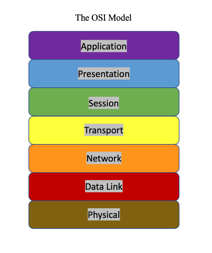
It is about time we introduce the OSI Model into our discussion of networking because in this blog, and especially in the next one, it is going to keep coming up in order to help us grasp networking signal flow on a conceptual level. The OSI Model or “Open Systems Interconnection Model” [1] is a conceptual model that educators use to break down the approach to networking into a hierarchy of 7 “levels of abstraction”, to use a term I borrowed from Carrie Ann Philbin’s “Crash Course Computer Science” Tutorials on YouTube [2]. (Sidebar: If you want to know more about how computers work, watch her video series because it’s amazing.)

The 7 Layers of the OSI Model

Let’s briefly break this down starting from the Physical layer and moving upward. At the very bottom at the Physical layer, this literally addresses the physical cable that you are using to plug one device into another. It also includes the binary bits or electrical signals that comprise the data we are moving around. As we move up a step, we arrive at the Data Link layer. The Lifeware article by Bradley Mitchell explains how this layer gets further subdivided into the “Logical Link Control” and “Media Access Control” layers as it is the “gatekeeper” that verifies data before it gets packaged [1]. Moving up from there, we arrive at the Network Layer and this is where data generally gets packaged, and the management involved in IP addressing falls in this realm. If the packages in the Network layer were cars, the Transport layer is where all the highways lie. This is where network protocols tend to fall in, but we will see in the next blog that it depends. Next up, I like to think of the Session layer like a session in your favorite digital audio workstation. This is where we start putting together these different highways and lower levels like taking a bunch of different audio tracks from different recordings and putting them together in one workspace. As we move up into the Presentation layer, this entails the methods that dictate how this data is going to be conveyed in the highest level at Application to the end user.  At the top of the model, we see the highest “level of abstraction” in Application. This is what the end user engages with, and by that I mean it is the most familiar way that we log in to a network. From now on, as we go through different aspects of our network design we are going to refer back to the OSI Model to help give us a reference of how these concepts work into the greater picture of our network design. Why are we going to do this? This is how we will think about the different steps of conceptualization that we will need to address (at least on some level) of our network design in order for it to work. The important thing to remember here is that even though we have all this granulation of detail available to visualize our network, manufacturers have put A LOT of money and research into making some of these levels simple for you to implement so that you (hopefully) don’t have to worry about them too much.

Down To The Wire

Now that our brains are primed with this level of abstraction, let’s talk about what cabling we can use for our network. In most networking applications, there are two major categories of cabling that you will likely encounter: copper and fiber. In the copper world, we often hear the terms “Ethernet”, “RJ45”, “Cat5”, “Cat5e”, and “Cat6” thrown around and used interchangeably as common types of network cabling. They often get used as misnomers instead of what they ACTUALLY refer to.

The term “Ethernet” actually doesn’t refer to a type of cable itself, it refers to a protocol called 802.3 as defined by the Institute of Electrical and Electronics Engineers (the IEEE, remember them from last time?) [3]. As mentioned in this Linksys article, Ethernet refers to “the most common type of Local Area Network (LAN) used today” [3]. (See how it’s all coming back around?) The most common types of cabling used for Ethernet includes the Cat5, Cat5e, and Cat6 specifications. The number refers to the generation of the cable [4]. The biggest differences between these three specifications is the bandwidth speeds these different specs can handle. This is a factor of the way the twisted pairs are wound inside the cable. The twisted pairs in Cat6 cabling are more tightly wound, which allows it to support higher bandwidths at higher transmission frequencies. This is also why how you coil these types of cables is so important as they lose efficiency if the twisted pairs become “unwound”. It also is a major drawback to the longevity of the cable itself and why it was originally intended for fixed installation. There are also stranded versus solid core versions of each cable, and while the advantage is that the solid core can transmit longer distances, it also is more susceptible to breakage.

Cat5, Cat5e, and Cat6 cable all contain four twisted pairs of conductors (hence the 8-pin connector) and can come in the form of UTP (Unshielded Twisted Pair) and STP (Shielded Twisted Pair). The idea being that a shielded twisted pair is less susceptible to outside interference, but it definitely ups the price point on the cable and MAY not be necessary depending on the application. For example, manufacturers often recommend shielded Cat5e or Cat6 cable for snakes for certain audio consoles to limit interference, but would that really be necessary for an installation in a home that is just getting a basic network set-up? Below is a table listing the major differences between Cat5, Cat5e, and Cat6 [5].

If you look at the jacket of a copper cable used for networking, you will probably see a marking listing one of these specifications. The 8-pin connector on the end of the cable is referred to as a RJ45 connector or “registered jack” [6] and is the most common networking plug.

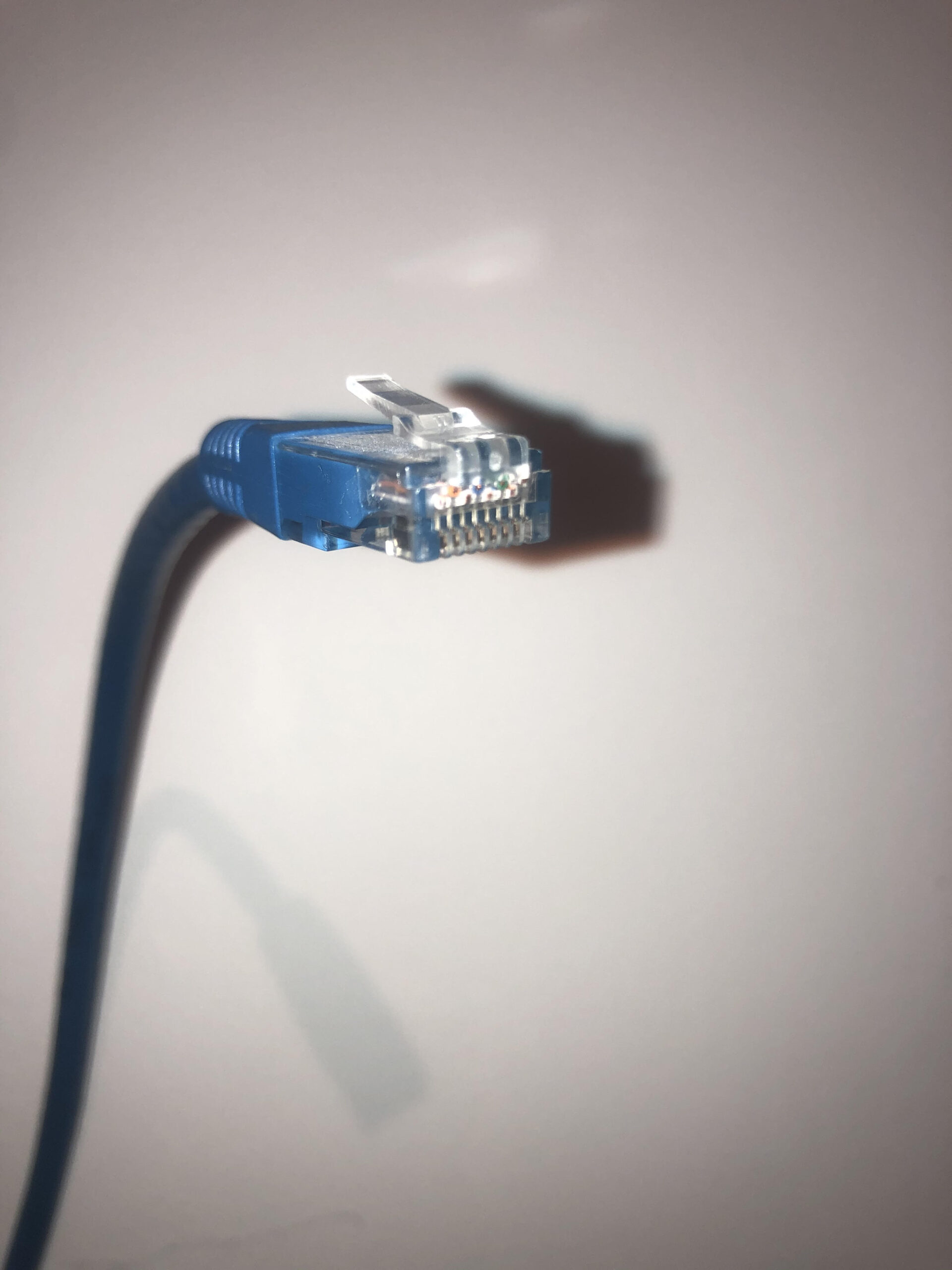
The end of a Cat6 patch cable with RJ45 connector. Notice the 8 conductors lined up with the 8 pins at the end.

Another major drawback of this copper cabling, besides the danger of the twisted pairs becoming “unwound” over time, is the length restriction. All 3 types of cabling are only rated to go a maximum of 100 meters, or roughly 330 feet, before needing a repeater or something to boost the signal again. This is where fiber wins by a longshot.

Another transport medium for data transmission involves converting the ones and zeros into light using a transceiver on both ends, and transferring it via fiber optic cabling. Fiber cabling is composed of single (or multiple) strands of glass or plastic roughly the diameter of a human hair [7]. The biggest advantage of fiber is its ability to go very long distances (depending whether it is singlemode or multimode fiber) with very little loss, very quickly. At the speed of light, in fact. The difference between singlemode and multimode fiber has to do with the thickness of the fiber core itself and how the light (which IS data) bounces around as it travels through the cable. In multimode fiber, the fiber core is larger and because it is larger, the light inside it bounces around the inside of the fiber more often. The Fiber Optic Association points out, the light travels “the core in many rays, called modes” [7]. These “refractions” inside the core cause some signal loss of the light over distance, which makes multimode relatively less efficient at traveling longer distances.

Singlemode vs Multimode fiber (including Grated-index and Step-index)

Singlemode fiber, on the other hand, has a significantly smaller core, which basically forces the light to travel in “only one ray (mode)” [7] allowing the signal to travel very long distances, we’re talking kilometers. This is an example of the type of fiber that might be used by your television company to send signals between cities. The problem with singlemode fiber is that while being expensive, it is also more delicate. It’s important to make the distinction here that the terms “singlemode” and “multimode” are related to the diameter/construction of the fiber core itself, NOT the number of strands in the fiber cable. There are military or “tactical grade” fiber cables with multiple strands of fiber in them like TAC-6 or TAC-12 that refer to the number of strands in the cable (6 and 12, respectively). You can have a TAC-6 or TAC-12 cable that can come in either singlemode or multimode flavors. In the majority of live sound applications, you will be dealing with multimode fiber, but before we move on, I want to make an important distinction about different types of fiber connectors.

The most common fiber connectors for live sound applications include LC and SC  (including single or duplex), and HMA or expanded beam connectors. SC connectors are a snap-in connection that have a 2.5mm ferrule, while LC is half the size with a 1.25mm ferrule [8]. These connectors are commonly seen in networking racks or from panels to stage racks as small yellow jumpers. They are cheap and, thus, they are delicate and can easily break if mishandled. The Neutrik opticalCON DUO cable [9] is based on LC-Duplex connectors, but the rugged build makes the connections more durable for the trials of live sound. Yet there is an important distinction here because these types of connectors care a lot more about alignment than an expanded beam connection.

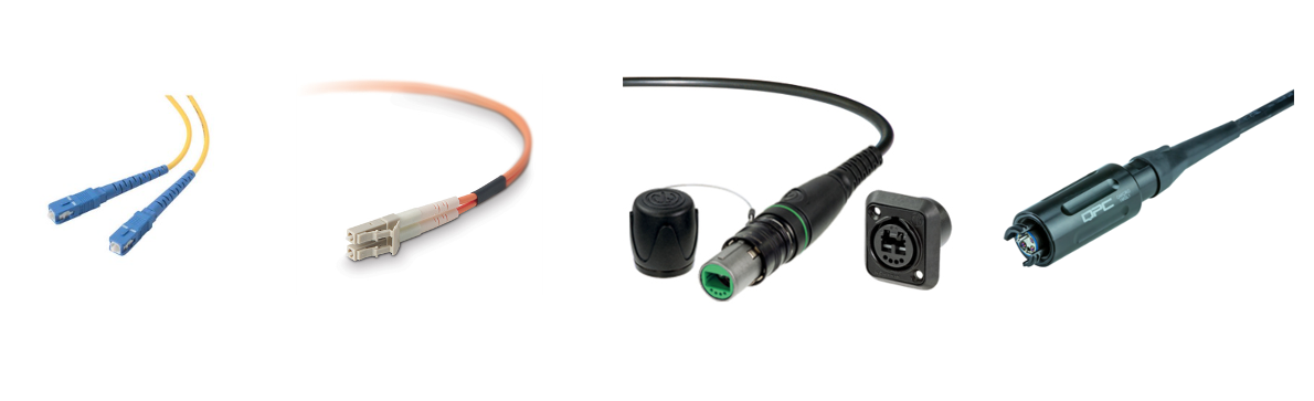
From left to right: L-Com SC-SC singlemode fiber cable [10], Belkin multimode fiber optic cable LC/LC duplex MMF [11], Neutrik opticalCON Duo [9], & QPC QMicro Expanded Beam Fiber optic connector [12] (I do not own the rights to these photos, for educational purposes only)

Once upon a time, in a world where we still did gigs on a regular basis, Sidney Wilson (the operations manager at Hi-Tech Audio in Hayward, California) sat down with me at the end of a day to explain to me how fiber optics worked. I was at Sound On Stage at the time, and our shop was just a stone’s throw away from the Hi-Tech shop so I went over after hours one day to ask him to teach me about fiber because, at the time, I knew nothing about it. He talked to me about the difference between the opticalCON-type fiber connectors and the HMA or expanded beam fiber connections. It has to do with the end of the fiber strand. On the SC and LC type connections, the end of the fiber is cut so that when you mate the connection, the alignment must be dead on in order to pass the light through. On the other hand, a HMA or expanded beam connection has a lens shaped like a ball on the connector that magnifies the light coming from the thin strand [12]. This makes the alignment of the connection more “forgiving” in terms of alignment since there is a greater surface area for contact. Consequently, this also makes the connector more lenient with the daily abuse of mating connections in the touring audio world, especially with the rugged, military-grade connector. The trade-off here is that there is SOME amount of loss due to the magnification of the lens.

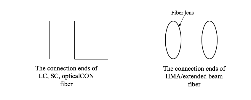
A simplified illustration comparing the mating of these two types of fiber ends. My attempt at recreating the napkin drawing Sidney originally drew to explain this to me.

So, as always, it comes down to application and, admittedly, the price tag. Leaving a box’s worth of Cat5e in a trench after a long corporate gig costs magnitudes less than trying to leave a single run of fiber after an event. Either way, whether we go with copper Cat5e cable or multimode HMA fiber, these transport mediums belong to the Physical layer of the OSI model, and deciding what to use for a given application is part of the basic decision making we need to assess in a network design.

“Papa, can you hear me?” → Message Transmission and Time

In the previous blog, I introduced the difference between unicast and multicast in the TCP/IP Protocol. We are now going to dig deeper and talk about how data gets transmitted, specifically in relation to time. First, let’s talk about the process called encapsulation. At the most basic level, a header and body is what composes a data packet. Pieces get added and/or stripped at different steps in the encapsulation process. In an article by Oracle, “the packet is the basic unit of information transferred across a network, consisting, at a minimum, of a header with the sending and receiving hosts’ addresses, and a body with the data to be transferred” [13]. The way to visualize the data encapsulation process of a TCP/IP Protocol Stack is like a consolidated version of the OSI model.

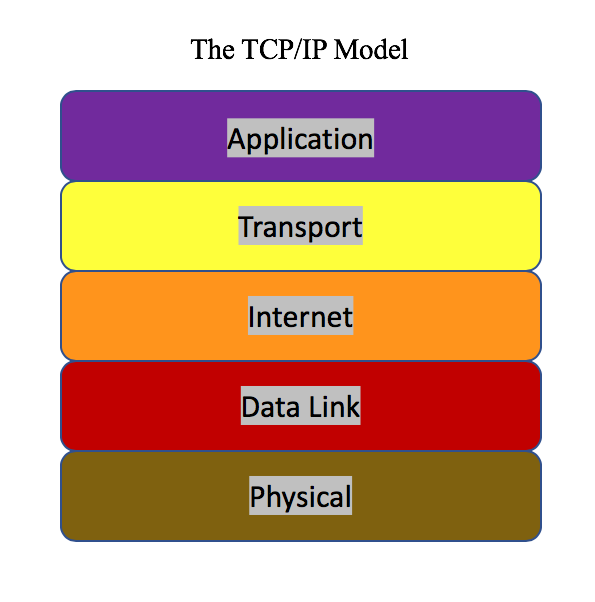
The TCP/IP Model looks like an abbreviated version of the OSI Model

At the Transport layer, depending on whether the packet uses UDP or TCP protocols, how the process passes off data changes in relation to accuracy and error checking. TCP, or Transmission Control Protocol [14], needs the start and endpoints of a transmission to acknowledge each other before passing data. In contrast, UDP, or User Datagram Protocol [15], does not check for this “handshake” when delivering packets and is widely used by audio-over-IP and higher-level protocols such as Dante. But why wouldn’t we want to use TCP that checks for errors since, after all, we need our data to be accurate? Well, the problem is that checking for these errors requires time. Audio, especially live, in-real-time applications require low latency, low time-delayed signal paths. A singer belting into a mic on a video screen and the audience hearing audio significantly later, generally doesn’t fly. If packets start getting lost or arriving at different times, this creates jitter in the data stream. So instead of choosing a protocol that goes back and “checks” to make sure all the data is there, in UDP we have chosen the path of least time resistance under the caveat that we better make sure it gets there. This is why QoS settings for UDP data transmission are very important.

If we were to set up a device, let’s say a managed switch, that will be dealing with UDP data transmission, we need to dive into the device’s administrative settings (or at least verify) that priority in the data transmission will be given to our time-sensitive data. QoS, or Quality of Service, refers to the management of bandwidth to prioritize certain data traffic over others. One example is DSCP, or Differentiated Services Code Point, which tags the packet header at the Network layer (in the OSI model) to prioritize that data in the transmission path [16]. If the network encounters a situation in which there is not enough bandwidth to pass all the data, the data without the priority tag gets queued until there is sufficient bandwidth to pass it, or it will get dropped first over the higher priority data [16]. For example, if you set up a classic Cisco SG300-10 managed switch to be used for Dante, part of the setup process is that you must log in to the administrator settings and set specific DSCP flags to prioritize data that is used for Dante over all other general network traffic. Once we start delving into these advanced settings such as QoS, we have to really keep in mind the overall picture of the function of our network. What is this data network going to be used for? Will we have other traffic like Internet traffic traveling alongside our audio signal? The capabilities of advanced networking allow us to accommodate all kinds of needs as long as we build and implement the network design properly.

Virtual Network Division (Boss-level)

One approach to taking a variety of network information and funneling it through to its various destinations is by utilizing VLANs and trunks. VLAN stands for “Virtual Local Area Network” and is basically what the name describes: it’s a way of creating a separated network that exists inside a greater network without having to do this physically. This is basically done at the Data Link layer by assigning certain ports on a managed switch to only carry certain broadcast domains. Here’s an example: say you have a network with two 10-port managed switches (one at either end) and you want Ports 1-4 to carry a VLAN (or multiple VLANs!) that is dedicated to the control network for running your favorite amplifier network controlling software, and then you want Port 5-8 to carry a VLAN (or multiple VLANs!) that has all audio-over-IP data. For the intentions of your network, you do not want these data streams to cross. By setting the switches up this way, you can use Ports 1-4 to plug in your laptop on one end to talk to the amplifiers on Ports 1-4 on the switch at the other end. Then other devices, say an audio console, can plug in anywhere on Ports 5-8 to pick up the data on the dedicated network that the stage rack is plugged in to on Port 5-8 on the switch at the other end. This is a great way of managing a large network to make sure that different devices don’t cross paths, but great care must be taken to make sure the correct settings are implemented and devices are plugged into the right ports in order to avoid a broadcast storm.

So how do all these separate VLANs get carried between the switches? It would kind of defeat the purpose of the VLAN to run separate cables between the switches connecting these ports. This is where trunking saves the day. Trunking involves the process of dedicating specific ports as “transport vehicles” to carry all the traffic from all the VLANs. Think of a trunk like a data version of a multicore snake carrying all the different, separated VLANs like separated, copper conductors on an analog snake. These are the connections you want to make between the managed switches. Be warned that generally, all network data travels through these ports so if you plug something into a trunk port that only wants to see traffic from a VLAN, it probably won’t be too happy about it. Here is a great way that, as a network designer, we can start harnessing the real power of our network. Some managed switches have certain SFP ports that allow for fiber connections using a special transceiver that converts data to light (and vice versa). Going back to our previous example, if Ports 9 and 10 are SFP ports and we set them up as trunks, we can run fiber for our cable path between switches and carry all our VLANs via that fiber connection. If you think about the possibility of utilizing multicore fiber cables such as TAC-6 or TAC-12 mentioned earlier so that each of those fibers contains a trunk that then carries multiple VLANs, it’s easy to see how the capabilities of our network quickly scale by orders of magnitude with these advanced setups. Now that we have conceptually seen how we can divide our network topology using VLANs and trunking, let’s take a step outward to see how we can divide it on a physical level.

Physical Network Division And Topologies

If you imagine a stage plot for a typical band and try to draw cable paths for all the snakes and sub snakes for each performer’s world, how you connect the stage boxes, to one another and/or to the main snakehead, will affect what will happen if there is some failure in one of the cables. The same concept applies when thinking about networks and how host devices or nodes connect to one another. In most live sound applications, there are four basic network topologies that you will encounter on a regular basis: daisy-chain, ring, star, and hybrid.

In a daisy-chain topology, we loop nodes from one device to the next in series. This is the most simple network to set up as it basically just involves connecting one device to another and then another and so on. Remember that the majority of network protocols implement a two-way road so the devices send and receive data back and forth on one cable. The problem with daisy-chaining your devices is that if one device goes down, it can take out your whole network depending on where it is in the signal path. It also adds more and more overall network latency as you go from one device to the next since we consider each node another hop in the network. In the example below, Console A is connected to Switch A, then to Rack A, and on to Rack B. If Rack A fails or a cable between Rack A and B fails, then Rack B gets taken down too because it is “downstream” of Rack A.

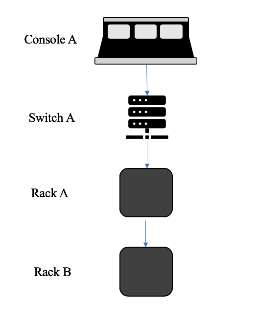
An example of a daisy-chain topology

If Rack A and Rack B had separate connections to Switch A, if one failed, the other would still have connection to the console.

In a star topology, one node acts as a hub in which other nodes branch off of it. This has less risk of one node failing and taking down the whole network. It has the disadvantage of using more cabling, but unless the node acting as the hub of the star goes down, it is far more resilient to individual host failures than the daisy-chain topology. In this example, we have connected a main switch in this rack to a series of networkable mic receivers. Yet instead of running a network cable to one receiver and then flowing through to daisy chain them together, we have run a separate cable from a discrete port on the switch to each receiver. Now if one receiver dies, regardless of where it is, we will still have network connection to the rest.

An example of a star topology

This also has the added advantage that the only network hop is from the hub device to the end node (or in this case, receiver). By using a combination of star and daisy-chain topology we have even more options.

A hybrid topology is a combination of utilizing several methods within the same network. Often this is necessary when you are incorporating devices with limited network ports, for making cable runs more efficient, and also lowering latency on big network deployments. Let’s say you are at a corporate event and have a console at FOH, but there is a stage rack in video world, two-stage racks in monitor world for the band inputs, and a rack in A2 world for wireless microphone receiver inputs. One possible solution utilizing a hybrid topology is to have the two-stage racks in monitor world daisy-chained from one to the other that then go to a switch that talks to both consoles in a star. Then the “master switch” talks to a switch in A2 world that has one port used by the wireless receivers daisy-chained together and then another port to the stage rack in video world because it is so close by.

An example of a hybrid topology in a network deployment

Now the “failure point” of this system is that if the switch in monitor world that acts like a hub for everything goes down, the whole network will pretty much go down with it. Maybe a possible solution would be to run a separate network connection from FOH to the switch in A2 world since the monitor engineer maybe is only there for the band portion of the event. It all comes down to designing the network with the least amount of failure points possible. As the joke goes in the world of audio: you can have cheap, efficient, and quality; pick two.

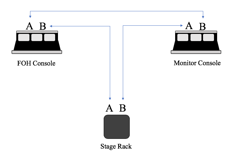
Another network topology worth mentioning here is called a ring. A ring network consists of devices that are always connected to two other neighboring devices.  In the world of live sound, we often see this from console manufacturers as a way for the console to always have one connection to a stage rack even if one of the two snake runs fail. In this example, the FOH and Monitor console are sharing one stage rack in a ring. On each device, or node, there is an “A” network connection and “B” network connection. In order to create a ring, cables make each connection as seen below from FOH port B to Stage Rack port A, Stage Rack port B to Monitor port A, and lastly back around from Monitor port B to FOH port A.

An example of a ring topology

Even if say the connection from FOH B to Stage Rack A somehow failed, since it is simultaneously still connected to Stage Rack B via the Monitor desk, the connection remains.

Daisy-chain, star, hybrid, and ring are very common network topologies in the world of live sound, but there are other topologies such as mesh networks that can be useful too, especially in wireless network applications. When you are designing your network it’s important to think about how you can make the system efficient given your situation’s requirements and available resources, without accumulating latency, and what level of redundancy you need the network to perform at.

Redundancy In The World Of Live Environments

Sidney Wilson also once pointed out to me that the level of redundancy we chose to abide by in the world of live sound is different than the expectations of redundancy in enterprise-level network applications. Let’s talk about the concepts of primary and secondary networks. As you might guess, the primary network is the main network path of data transmission, while the secondary network is your back-up in case something happens to the primary. This can range from having devices with the capability to maintain two internally separated networks to having two entirely separate rigs, consoles and all, in case the primary goes down. In an enterprise-level network installation, they might run separate cables down completely separate paths of the building to prevent the network from going down if one cable fails. Yet in the world of live sound, and especially touring applications, how often do we run two separate cable paths for the audio snake to FOH? One for the primary run, one to the secondary? Maybe if it is important enough, you might be able to run the snakes on two separate paths. Yet if you were at a music festival where there is one snake path for everyone because of cable jackets and safety precautions, the chances of you being able to do that is pretty close to nil. So, like everything in the live entertainment industry, it is a game of compromise.

What’s really cool is that you can apply this concept of redundancy to almost every level of the OSI model. Technology keeps improving to give us more failsafes in our network design. On the one hand, you can have physically separate cable runs and/or systems for a primary and secondary network, and if one fails then someone literally unplugs the main data stream into the secondary network. There are also different protocols that implement redundancy by having “automatic” switchovers where if the primary network fails, the data switches almost instantaneously to the secondary network. This includes Dante and AVB networks with Milan.

If you’ve made it this far, congratulations! Thank you for sticking with me through these first two blogs from explanations of binary to the extensive discussion of network cable. If you’ve read the last blog and this one, my hope is that you can combine the knowledge from the two to start conceptualizing how all these pieces work together in the application of the world of live sound. Now that we have established this basis in which to talk about networking, in the next blog we will advance into the world of networking protocols such as AVB and Dante. Now that we have this knowledge under our belt we can better compare and contrast the applications and usages for both. See you next time!

*I thought this name covered this concept a lot better than “Dividing A Network” as mentioned at the end of my last blog

Endnotes

[1] https://www.lifewire.com/layers-of-the-osi-model-illustrated-818017

[2] https://www.youtube.com/playlist?list=PL8dPuuaLjXtNlUrzyH5r6jN9ulIgZBpdo

[3] https://www.linksys.com/us/r/resource-center/basics/whats-ethernet/

[4]https://medium.com/@cloris326192312/what-is-the-difference-between-cat5-cat5e-and-cat6-cable-530e4e0ab12b

[5] http://ciscorouterswitch.over-blog.com/article-cat5-vs-cat5e-vs-cat6-125134063.html

[6] https://techterms.com/definition/rj45

[7] https://www.thefoa.org/tech/ref/basic/fiber.html

[8] https://www.thefoa.org/tech/connID.htm

[9]https://www.neutrik.com/en/neutrik/products/opticalcon-fiber-optic-connection-system/opticalcon-advanced/opticalcon-duo/opticalcon-duo-cable

[10] https://www.l-com.com/fiber-optic-9-125-singlemode-fiber-cable-sc-sc-30m

[11] https://www.belkin.com/us/p/P-F2F202LL/

[12] https://www.qpcfiber.com/product/qmicro/

[13] https://docs.oracle.com/cd/E19455-01/806-0916/ipov-32/index.html

[14] https://www.pcmag.com/encyclopedia/term/tcp

[15] https://www.pcmag.com/encyclopedia/term/udp

[16] https://www.networkcomputing.com/networking/basics-qos

Resources:

Audinate. (n.d.). Dante Certification Program. https://www.audinate.com/learning/training-certification/dante-certification-program

Audio Technica U.S., Inc. (2014, November 5). Networking Fundamentals for Dante. https://www.audio-technica.com/cms/resource_library/files/89301711029b9788/networking_fundamentals_for_dante.pdf

Belkin International, Inc. (n.d.). Belkin Fiber Optic Cable; Multimode LC/LC Duplex MMF, 62.5/125. Retrieved June 21, 2020 from https://www.belkin.com/us/p/P-F2F202LL/

Cai, Cloris. (2016, December 29). What Is The Difference Between Cat5, Cat5e, and Cat6 Cable?. Medium. https://medium.com/@cloris326192312/what-is-the-difference-between-cat5-cat5e-and-cat6-cable-530e4e0ab12b

Chapman, B.D. & Zwicky, E.D. (1995, November). Building Internet Firewalls. O’Reilly & Associates. http://web.deu.edu.tr/doc/oreily/networking/firewall/ch06_03.htm

Cisco & Cisco Router, Network Switch. (2014, December 3). CAT5 vs. CAT5e vs. CAT6. Overblog. http://ciscorouterswitch.over-blog.com/article-cat5-vs-cat5e-vs-cat6-125134063.html

Crash Course. (2020, March 19). Computer Science [Video Playlist]. YouTube. https://www.youtube.com/playlist?list=PL8dPuuaLjXtNlUrzyH5r6jN9ulIgZBpdo

Froehlich, Andrew. (2016, August 15). The Basics of QoS. Network Computing. https://www.networkcomputing.com/networking/basics-qos

Geeks for Geeks. (n.d.). Types of Network Topology. Retrieved June 21, 2020 from https://www.geeksforgeeks.org/types-of-network-topology/

Infinite Electronics International, Inc. (n.d.) 9/25, Singlemode Fiber Cable, SC / SC, 3.0m. L-com. Retrieved June 21, 2020 from https://www.l-com.com/fiber-optic-9-125-singlemode-fiber-cable-sc-sc-30m

Linksys. (n.d.). What is Ethernet?. Retrieved June 21, 2020 from https://www.linksys.com/us/r/resource-center/basics/whats-ethernet/

Mitchell, Bradley. (2020, April 29). The Layers of the OSI Model Illustrated. Lifewire. https://www.lifewire.com/layers-of-the-osi-model-illustrated-818017

Neutrik. (n.d.). OpticalCON DUO Cable. Retrieved June 21, 2020 from https://www.neutrik.com/en/neutrik/products/opticalcon-fiber-optic-connection-system/opticalcon-advanced/opticalcon-duo/opticalcon-duo-cable

Oracle Corporation. (2010). Data Encapsulation and the TCP/IP Protocol Stack. In System Administration Guide, Volume 3. Retrieved June 21, 2020 from https://docs.oracle.com/cd/E19455-01/806-0916/ipov-32/index.html

PCMag. (n.d.). TCP. In PCMag Encyclopedia. Retrieved June 21, 2020 from https://www.pcmag.com/encyclopedia/term/tcp

PCMag. (n.d.). UDP. In PCMag Encyclopedia. Retrieved June 21, 2020 from https://www.pcmag.com/encyclopedia/term/udp

QPC. (n.d.). QMicro. Retrieved June 21, 2020 from, https://www.qpcfiber.com/product/qmicro/

TechDifferences. (2017, August 18). Difference Between Frame and Packet. https://techdifferences.com/difference-between-frame-and-packet.html

Tech Terms. (2011, July 1). RJ45. https://techterms.com/definition/rj45

The Fiber Optic Association, Inc. (2019). Guide To Fiber Optics & Premises Cabling. Retrieved June 21, 2020 from https://www.thefoa.org/tech/connID.htm

The Fiber Optic Association, Inc. (2018). Reference Guide. Retrieved June 21, 2020 from https://www.thefoa.org/tech/ref/basic/fiber.html