La fase y el filtro de peine
“La suma es una forma de juego acústico donde la amplitud relativa fija la apuesta y la fase relativa decide al ganador.”
– Bob McCarthy
A lo largo de este articulo hablaremos sobre que es la fase y como es que afecta nuestras mediciones. Estos conceptos nos darán claridad en qué posición usar nuestro micrófono de medición, con estas técnicas logro conseguir grandes resultados en mis mediciones.
Qué es la fase?
La fase está relacionada al tiempo, aunque debemos tomar en cuenta que no es la única variable que puede modificar la fase.
Para tener más claro de que trata la fase debemos recordar que el periodo (T) es el tiempo que le toma a una onda desenvolver un ciclo completo de una determinada frecuencia. Matemáticamente:
T (segundos) =1sfrecuencia o T(milisegundos)=1000ms/frecuencia
Es importante tomar en cuenta que para las frecuencias audibles (20 Hz – 20,000 Hz) hay una relación de 1:1,000. Esto significa que el periodo de 20 Hz (50 ms) es mil veces mayor al de 20,000 Hz (0.05ms).
Tomando en cuenta estos detalles entremos en materia.
Si pensamos en una onda senoidal y en su semejanza con un círculo “desdoblado”, pensaríamos que podemos expresar en qué posición de la onda senoidal nos encontramos por medio de grados.
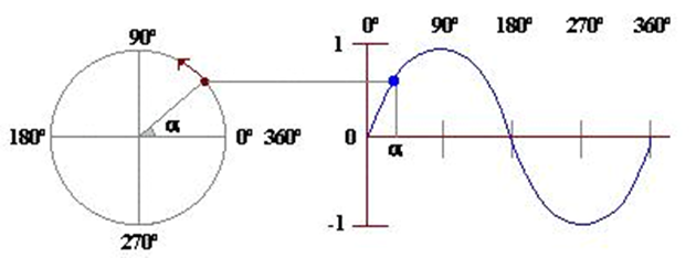
Siendo 0° el inicio de la onda, 90° el valor de máxima amplitud, 180° media onda, 270° la mínima amplitud y 360° el fin de un ciclo completo (y el inicio del siguiente).
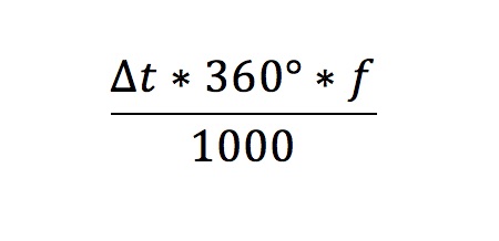
Pensando en esto podemos asociar la fase y la amplitud de una onda al tiempo. Veamos la siguiente expresión.
Siendo:
ΔØ la fase resultante
Δt el tiempo en el que se hace el análisis (en milisegundos)
f la frecuencia
Pensando en esta expresión matemática podemos darnos cuenta que la fase es directamente proporcional a la frecuencia y al tiempo transcurrido. Hagamos un análisis de que sucede con la fase si pasa 1 ms desde que inicia una señal.
Fase resultante después de 1 ms:
100 Hz = 36°
500 Hz = 180°
1,000 Hz = 360°
1,500 Hz = 540°
2,000 Hz = 720°
10,000 Hz = 3,600°
La fase nos ayuda a saber cuántos ciclos o fracciones de ciclo han pasado al transcurrir un determinado tiempo. Cabe resaltar que la fase es una característica de las ondas y no es necesario que haya más de una señal para poder hacer un análisis al respecto.
Qué ocurre cuando interactúan 2 señales?
Hasta ahora hemos hablado de la fase en una sola señal y esto no parece tener mayor complicación, me atrevo a decir que mucho de nosotros incluso no recordamos que la fase existe hasta que no tenemos más de una señal correlacionada interactuando. La relación de fase entre 2 señales correlacionadas determina cual será el resultado de la suma de dichas señales.
Hagamos un ejercicio.
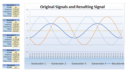
Vamos a usar 2 generadores de tonos para generar en ambos 1,000 Hz con una amplitud de 0dB.
Veremos en un osciloscopio las señales de los generadores y la suma de ambas señales.
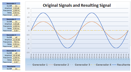
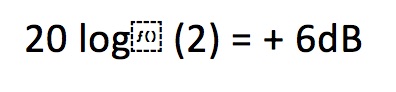
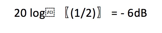
En esta imagen podemos observar que ambos generadores tienen la misma amplitud y la misma fase. Si observamos la curva “Resultante”, que es la suma de ambas señales, podemos notar como la amplitud se ha duplicado. Si expresamos el resultado en dBs diríamos que:
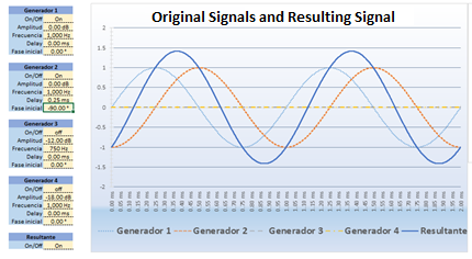
En esta imagen podemos observar que hay una diferencia de fase de 90° entre las señales. Si observamos la curva “Resultante” podemos notar como la amplitud ha sumado solo hasta 1.41 y que la fase de la señal resultante ha tomado el valor medio entre ambas señales. Si expresamos el resultado en dBs diríamos que:

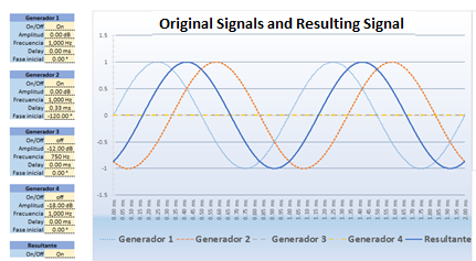
En esta imagen podemos observar que hay una diferencia de fase de 120° entre las señales. Si observamos la curva “Resultante” podemos notar como la amplitud no ha sumado nada y que la fase de la señal resultante ha tomado el valor medio entre ambas señales. Si expresamos el resultado en dBs diríamos que:

En esta imagen podemos observar que hay una diferencia de fase de 150° entre las señales. Si observamos la curva “Resultante” podemos notar como la amplitud se ha atenuado hasta 0.5 y que la fase de la señal resultante ha tomado el valor medio entre ambas señales. Si expresamos el resultado en dBs diríamos que:
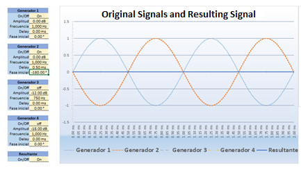
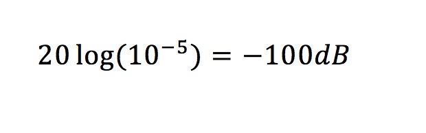
En esta imagen podemos observar que hay una diferencia de fase de 180° entre las señales. Si observamos la curva “Resultante” podemos notar como la amplitud se ha cancelado por completo. Si expresamos el resultado en dBs diríamos que:
De todo esto podemos concluir que la suma de 2 señales correlacionadas está estrechamente ligada a la relación de fase que hay entre ambas señales. Este comportamiento se resume en la siguiente ecuación.
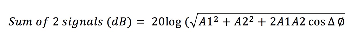
Donde:
A1 = Amplitud de la señal 1
A2 = Amplitud de la señal 2
Δ∅ = Diferencia de fase entre las señales
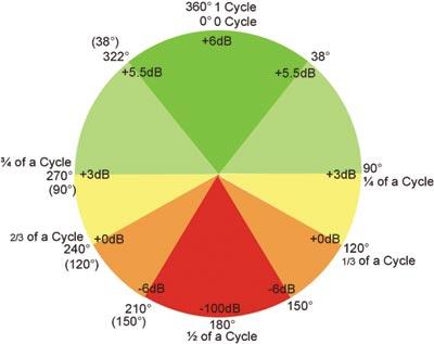
Y se resume visualmente en el círculo de fase.
El filtro de peine
En los ejercicios anteriores comprendimos cómo es que la fase determina si hay suma o cancelación al sumar 2 señales, pero debemos tomar en cuenta que en estos ejercicios trabajamos únicamente con tonos senoidales, es decir una sola frecuencia. La realidad es que nosotros no trabajamos con tonos senoidales, ahora debemos analizar que sucede con señales de espectro completo.
Veamos el siguiente ejemplo:
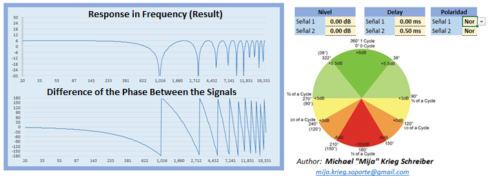
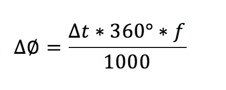
En esta imagen podemos apreciar la suma de 2 señales de espectro completo. Estas señales tienen una diferencia de tiempo de 0.5 ms, que es el periodo de 2,000 Hz. Sabemos que esta diferencia de tiempo afectara de manera diferente a cada frecuencia, veamos algunos ejemplos:
Δ∅=t*360°*f/1000
Δ∅ @500 Hz = 90° (+3dB de suma).
Δ∅ @1,000 Hz = 180° (-100dB de atenuación).
Δ∅ @2,000 Hz = 360° (+6dB de suma).
Δ∅ @3,000 Hz = 540° (-100dB de atenuación).
Δ∅ @4,000 Hz = 720° (+6dB de suma).
Este fenómeno es conocido como filtro de peine, llamado así por la semejanza del grafico a un peine.
Cómo afecta el filtro de peine nuestras mediciones?
Sabemos que el filtro de peine es el resultado de sumar 2 señales correlacionadas con diferencias de tiempo. Cuando realizamos mediciones en campo hay muchas posibles causas del filtro de peine, una de estas causas son las reflexiones.
Podemos imaginar las reflexiones como una imagen fantasma de la señal original pero retrasada en tiempo. La señal reflejada recorre mayor distancia, esto es lo que causa el retraso.
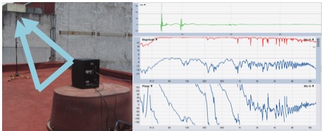
Veamos este ejemplo realizado con un micrófono de medición MM1 de Beyerdynamics y un altavoz de rango completo.
En esta imagen podemos apreciar como la señal directa y la señal reflejada llega al micrófono con diferencia de tiempo. Por medio de la respuesta impulsiva podemos averiguar que la diferencia de tiempo es de 1.67 ms, que es el periodo de 600 Hz. Veamos que sucede en algunas frecuencias al agregar 1.67 ms de diferencia.
Δ∅ @300 Hz = 180° (cancelación)
Δ∅ @600 Hz = 360° (suma)
Δ∅ @900 Hz = 540° (cancelación)
Etc…
Cómo podemos disminuir el filtro de peine en la reflexión?
Ya está claro que el filtro de peine es causado por la diferencia de tiempo entre ambas señales, si queremos eliminar el filtro de peine podríamos:
- Eliminar la reflexión, podríamos lograr eso quitando el piso o dándole tratamiento acústico. Esta opción no es posible.
- Minimizar la diferencia de tiempo, podríamos lograr esto al disminuir la diferencia en el recorrido de la señal reflejada respecto a la señal directa.
En esta imagen podemos ver cómo hemos logrado mejorar nuestra medición con tan solo colocar el micrófono en el piso. Estas mediciones son conocidas como “Ground plane”.
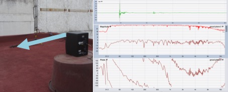
Esta medición no elimina la reflexión, en lugar de eso nos hemos acercado tanto a la reflexión que no logramos ver la diferencia de tiempo entre esta y la señal original.
Este tipo de mediciones son de gran ayuda cuando trabajamos en lugares con superficies muy reflejantes, nos permiten centrar la atención en lo que realmente está haciendo el sistema de altavoces. Claro que una persona que esté de pie segura notando la presencia del filtro de peine, pero cuando el recinto este lleno de personas el mismo coeficiente de absorción acústica de los espectadores evitara que la reflexión pueda causar filtros de peine.
Preguntas:
Qué indica la fase?
- El avance o posición de una onda senoidal expresada en grados
- La diferencia de tiempo entre 2 altavoces
- El periodo de una señal
- La polaridad de una señal
Cuál es el resultado de sumar 2 tonos con la misma amplitud pero una diferencia de fase de 90°?
- +3dB
- +6dB
- 0dB
- -3dB
Cuál es el resultado de sumar 2 tonos con la misma amplitud pero una diferencia de fase de 180°?
- 0dB
- -6dB
- -100dB
- No se puede saber
Qué es el filtro de peine?
- Es la inducción causada por no peinar adecuadamente el cableado
- Es el resultado de sumar 2 señales correlacionadas con una diferencia de tiempo
- Es el resultado de sumar 2 señales no correlacionadas con una diferencia de tiempo
- Es el resultado de sumar 2 señales correlacionadas con una inversión de polaridad
En que consisten las mediciones “Ground plane”?
- En reducir la diferencia de tiempo entre la señal directa y la señal reflejada en una medición.
- Se trata de la medición del ruido que captaran las hormigas durante el show.
- Quitar las reflexiones de la medición
- Reducir la interferencia causada por el viento
 Michael “Mija” Krieg Schreiber
Después de que en el 2010 obtuvo un grado en Técnico en Audio, con la especialidad de audio en vivo, tomó una serie de cursos relacionados a la materia, tales como el uso y aplicación del software Smaart, arreglos lineales, diseño de sistemas de refuerzo sonoro, SIM3, procesadores de arquitectura abierta, entre muchos otros.
Ha trabajado en diversas compañías, producciones, discotecas e instalaciones como instructor, diseñador, técnico y operador de sistemas de sonido reuniendo a la fecha 9 años de experiencia. Entre las compañías, producciones y recintos con los que ha trabajado se encuentran Representaciones de Audio, Meyer Sound México, Hi tech Audio, la Misa papal en San Cristóbal de las Casas 2016, Corona Capital 2014, Auditorio Nacional, Arena Ciudad de México, entre otros.
Hoy en día concentra su carrera en actividades educativas ofreciendo diferentes ponencias y cursos de audio profesional. Entre las escuelas y organizaciones con las que ha colaborado están: Avixa, AES México, Instituto Politécnico Nacional, Instituto Tecnológico y de Estudios Superiores de Monterrey, UNITEC Universidad Tecnológica de México, SAE INSTITUTE México, EMEH Escuela de la Música del Estado de Hidalgo, G Martell, Pro Audio Puebla, entre otras.