Part Three: Networking Protocols

(or A History of IEEE Standards)

Read Part One Here

Read Part Two Here

Evaluating Applications

One thing I have learned from my do-it-yourself research in computer science that I have applied to understanding the world in general is the concept of building on “levels of abstraction.” (Once again, here I am quoting Carrie Ann Philbin from the “Crash Course: Computer Science” YouTube series) [1]. From the laptop that this blog was written on, to performing a show in an arena, all these things would not be possible if it were not for the multitude of smaller parts working together to create a system. Whether it is an arena concert divided into different departments to execute the gig or a data network broken up into different steps in the OSI Model, we can take a complicated system and break it down into its composite parts to understand how it works as a whole. Similarly, the efficiency and innovation of this compartmentalization in technology lays in the fact that one person can work on just one section of the OSI Model (like the Transport Layer) while not really needing to know anything about what’s happening on the other layers.

This is why I have spent all this time in the last two blogs of “Basic Networking For Live Sound Engineers” breaking up the daunting concept of networking into smaller composites from defining what is a network to designing topologies including VLANS and trunks. At this point, we have spent a lot of time talking about how everything from Cat6 cable to switches physically and conceptually works together. Now it’s time to really dive deep into the languages, or protocols, that these devices use to transmit audio. This is a fundamental piece in deciding on a network design because one protocol may be more appropriate for a particular design versus another. As we discuss how these protocols handle different aspects of a data packet differently, I want you to think about why one might be more beneficial in one situation versus another. After all, there are so many factors that go into the design of a system from working in pre-existing infrastructures to building networks from scratch, that we must take these variables into account in our network design decisions. A joke often appears in the world of live entertainment: you can have cheap, efficient, or quality. Pick 2.

What Is In A Packet, Really?

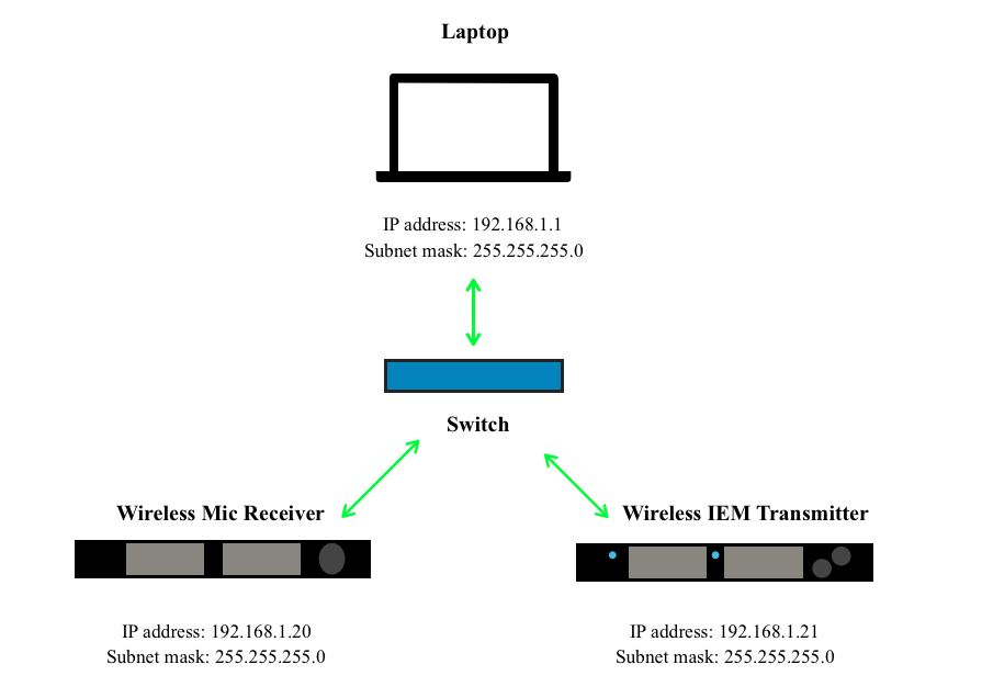
As a quick refresher from Part 2, data gets encapsulated in a process that involves the formation of a header and body for each packet. The very basic overall structure of a packet or frame includes a header and body. How you define each section and whether it is actually called a “packet” or “frame” depends on what layer of the OSI Model you are referring to.

Basic structure of a data packet…or do I mean frame? It depends!!

Now this back and forth of terminology seemed really confusing until I read a thread in StackExchange that pointed out that the “combination” of the header and data at Level 2 is called a frame and at Level 3 is called a packet [2]. The change in terminology corresponds to different additions in the encapsulation process at different layers in the OSI Model.

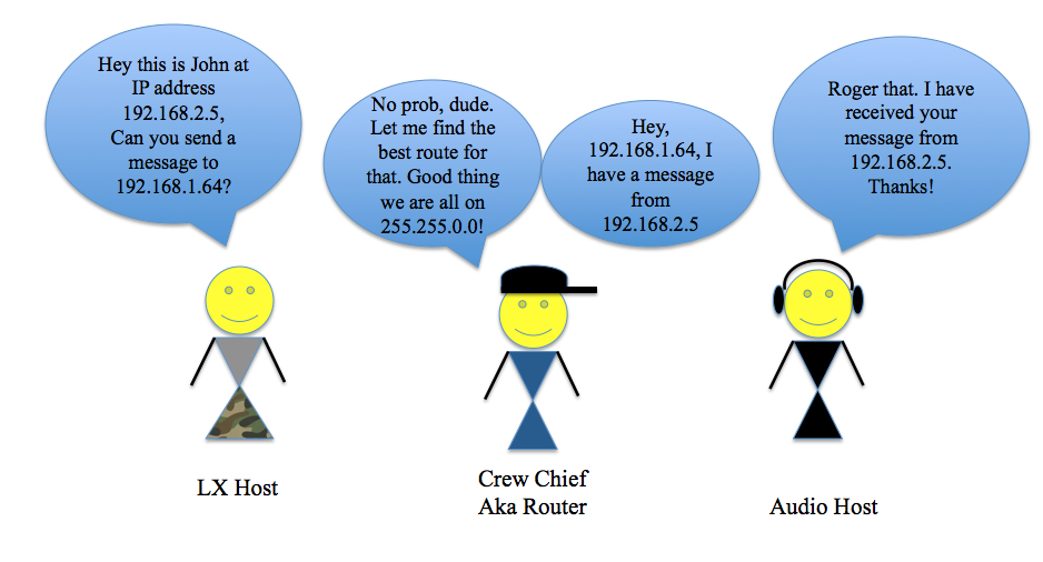
In an article by Alison Quine on “How Encapsulation Works Within the TCP/IP Model,” the encapsulation process involves adding headers onto a body of data at each step starting from the top of the OSI model at the Application layer and moving down to Physical Layer, and then stripping off each of those headers as you move back up the OSI Model in reverse through each process [3]. That means that during the encapsulation process at each parameter within the OSI Model for a given network, there is another header that gets added on to help the data get to the right place. Audinate’s Dante Level 3 training on “IP Encapsulation” talks about this process in a network stack. At the Application level, we start with a piece of data. Then at the Transport Layer, the source port, destination port, and the transport protocol attach to the data or payload. At the Network Layer, the Destination and Source IP address add on top of what already exists in the Transport Layer. Then at the Data Link layer, the destination and source MAC addresses attach on top of everything else in the frame by referencing an ARP table [4]. ARP, or Address Resolution Protocol, uses message requests to build tables in devices (like a switch, for example) to match IP addresses to MAC addresses, and vice versa.

So I want to pause for a second before we move onward to really drive the point home that the OSI Model is a conceptual tool used for educational purposes to talk about different aspects of networking. For example, you can use the OSI Model to understand network protocols or understand different types of switches. The point is we are using it here to understand the signal flow in the encapsulation process of data, just as you would look at a chart of signal flow for a mixer.

Check 1, Check 2…

There is the old visage that time equals money, but the reality of working in live sound is that time is of the essence. Lost audio packets that create jitter or sound audibly delayed (our brains are very good at detecting time differences) are not acceptable. So it goes without saying that data has to arrive as close to synchronously as possible. In my previous blog on clocks, I talked about the importance of different digital audio devices starting their sampling at the same rate based on a leader clock (also referred to as a master clock) in order to preserve the original waveform. An accurate clock is important in preserving the word length, or bits, of the data. Let’s look at this example:

1010001111001110

1010001111001110

In this example, we have two 16 bit words which represent two copies of the same sample of data traveling between two devices that are in sync because of the same clock. Now, what happens if the clock is off by just one bit?

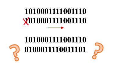
If the sample is off by even just one bit, the whole word gets shifted and produces an entirely different value altogether! This manifests itself as digital artifacts, jitter, or no signal at all. So move up a “level of abstraction” to the data packet at the Network level in the OSI Model and you can understand why it is important for packets to arrive on time in a network so that bits of data don’t get lost or packets don’t collide because otherwise, it will create a broadcast storm. But as I’ve mentioned before, UDP and TCP/IP handles data accuracy and timing differences.

Recall from Part 2 that TCP/IP checks for a “handshake” between the receiver and sender to validate the data transmission at the cost of time, while UDP decreases transmission time in exchange for not doing this back and forth validation. In an article from LearnCisco on “Understanding the TCP/IP Transport Layer,” TCP/IP is a “connection-oriented protocol” that requires adding more processes into the header to verify the “handshake” between the sender and receiver [5]. On the other hand, UDP acts as a “connectionless protocol”:

[…] there will be some error checking in the form of checksums that go along with the packet to verify integrity of those packets. There is also a pseudo-header or small header that includes source and destination ports. And so, if the service is not running on a specific machine, then UDP will return an error message saying that the service is not available. [5]

So instead of verifying that the data made it to the destination, UDP will check that the packet’s integrity is solid and if there is a path available for it to take. If there is no available path, the packet just won’t get sent. Due to the lack of “error checking” in UDP, it is imperative that the packets arrive at their correct destination and on time. So how does a network actually keep time? In reference to what?

Time, Media Clocking, and PTP

Let’s get philosophical for a moment and talk about the abstraction of time. So I have a calendar on my phone that I schedule events and reminders based on a day divided into hours and minutes. This division of hours and minutes are arguably pointless without being referenced to some standard of time, which in this case is the clock on my phone. I assume that the clock inside my phone is accurate in relation to a greater reference of time wherever I am located. The standard for civil time is UTC or “Coordinated Universal Time” which is a compromise between the TAI standard, based on atomic clocks, and UT1, which is based on an average solar day, by making up for it in leap seconds [6]. In order for me to have a Zoom call with someone in another time zone, we need a reference to the same moment wherever we are because it doesn’t matter if I say our Zoom call is at 12 pm Pacific Standard Time and they think it is at 3 pm Eastern Standard Time as long as our clocks have the same ultimate point of reference, which for us civilians is UTC. In this same sense, digital devices need a media clock with reference to a common master (but we are going to update this term to leader) in order to make sure data gets transmitted without bit-slippage as we discussed earlier.

In a white paper titled “Media Clock Synchronization Based On PTP” from the Audio Engineering Society 44th International Conference in San Diego, Hans Weibel and Stefan Heinzmann note that, “In a networked media system it is desirable to use the network itself for ensuring synchronization, rather than requiring a separate clock distribution system that uses its own wiring” [7]. This is where PTP or Precision Time Protocol comes in. The IEEE (Institute of Electrical and Electronics Engineers) 1588 standardized this protocol in 2002, and expanded it further in 2008 [7]. The 2002 standard created PTPv1 that works using UDP on a level of microsecond accuracy by sending sync messages between leader and follower clocks. As described in the Weibel and Heinzmann paper, on the Application layer follower nodes compare their local clocks to the sync messages sent by the leader and adjust their clocks to match while also taking into account the absolute time offset in the delay between the leader and follower [7]. Say we have two Devices A and B:

Device A (our leader for all intents and purposes) sends a Sync message to Device B saying, “This is what time it is. 11:00 A.M.”

Device B says, “Ok. I think it’s 12:00 P.M,” This is the Follow_Up message.“What time did you send that message?” says the Delay_Request message.

Device A replies, “At 11:00 A.M.” This is the Delay_Response message. “What time did you receive it?”

Device B replies, “At 12:15 P.M. Ok, I’ll adjust.”

Analogy of clocking communication in PTPv1 as described in IEEE 1588-2002

This back and forth allows the follower to adjust their clocks to whatever clock is considered the leader according to the best master clock algorithm (which should be renamed the best leader clock algorithm) and the ultimate reference being considered the grandmaster clock/grandleader clock [8]. Fun fact: in the Weibel and Heinzmann paper, they point out that “the epoch of the PTP time scale is midnight on 1 January TAI. A sampling point coinciding with this point in absolute time is said to have zero phase” [9].

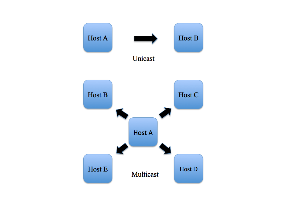
So in 2008, the standards got updated to PTPv2, which of course is not backwards compatible with PTPv1 [10]. But this update includes changing how clock quality is determined, going from all PTP messages being multicast in v1 to having the option of unicast in v2, improving clocking accuracy from microseconds to nanoseconds, and the introduction of transparent clocks. The 1588-2002 standard introduced the concept of ordinary clocks as a device or clock node with one port while boundary clocks have two or more ports [11]. Switches and routers can be an example of a boundary clock while other end-point devices including audio equipment can be examples of ordinary clocks. A Luminex article titled “PTPv2 Timing protocol in AV Networks” describes how “[a] Transparent Clock will calculate how long packets have spent inside of itself and add a correction for that to the packets as they leave. In that sense, the [boundary clock] becomes ‘transparent’ in time, as if it is not contributing to delay in the network” [12]. PTPv2 improves upon the Sync message system by adding an announce message scheme for electing the grandmaster/grandleader clock. The Luminex article illustrates this by describing how a PTPv2 device starts up in a state “listening” for announce messages that include information about the quality of the clock until a determined amount of time called the Announce Timeout Interval. If no messages arrive, that device becomes the leader. Yet if it receives an announce message indicating the other clock has superior quality, it will revert to a follower and make the other device the leader [13]. It is these differences in the handling of clocking between IEEE 1588-2002 and 2008 that will be key to understanding the underlying difference when talking about Dante versus AVB.

Dante, AVB, AES67, RAVENNA, and Milan

Much like the battles between Blu-Ray, HD DVDs, and other contending audiovisual formats, you can bet that there has been a struggle over the years to create a manufacturer-independent standard for audio-over-IP or networking protocols used in the audio world. The two major players that have come out on top in terms of widespread use in the audio industry are AVB and Dante. AES67 and RAVENNA are popular as well, RAVENNA dominating the world of broadcast.

Dante, created by the company Audinate, began in 2003 under the key principle that still makes the protocol appealing today: the ability to use pre-existing IT infrastructures to distribute audio over a network [14]. Its other major appeal is that it allows for use of redundancy that makes it particularly appealing to the world of live production. In a Dante network you can set up a primary and secondary network, the secondary being an identical “copy” of the primary so that if the primary network fails, it switches over seamlessly to the secondary. Dante works at the Network Layer (Layer 3) of the OSI Model by resting on top of the IP addressing schemes already in place in a standard IT networking system and works above this. It’s understandable financially why a major corporate office would want to use this protocol because of the savings on overhauling the entire infrastructure of an office building to put in new switches, upgrade topologies, and so on.

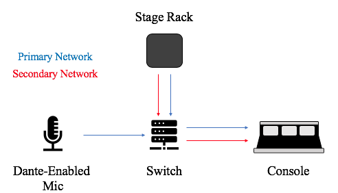
An example of a basic Dante Network with redundant primary (blue) and secondary (red) networks

The adaptable nature of Dante comes from existing as a Layer 3 protocol, which allows one to use most Gigabit switches and even sometimes 100Mbps switches to distribute a Dante network (but only if it’s solely a 100Mbps network) [15]. That being said, there are some caveats. It is strongly recommended (and in 100Mbps networks, mandatory) to use specific Quality of Service (QoS) settings when configuring managed switches (switches whose ports and other features are configurable usually via a software GUI) to be used for Dante. This includes flagging specific DSCP values that are important to Dante traffic as high priority, including our friend PTP. Other network traffic can exist alongside Dante traffic on a network as long as the subnets are configured correctly (for more info on what I mean by subnets, see Part 1 of this blog series). I myself personally prefer configuring specific VLANs for dedicated network control traffic and Dante to keep the waters clear between the two. This is because I know control network traffic will not be prioritized over Dante traffic because of QoS, but at the same time Dante was made for this so as long as your subnets are configured correctly, it should be fine. The issue is that with Dante using PTPv1, even with proper QoS settings the clock precision can get choked if there are issues with bandwidth. The Luminex article mentioned earlier discusses this: “Clock precision can still be affected by the volume of traffic and how much contention there is for priority. Thus; PTP clock messages can get stuck and delayed in the backbone; in the switches between your devices” [16].

So since Dante uses PTPv1, Dante will find the best device on the network to be the Master (Leader) Clock using PTP as the clocking system for the entire network, and if one device drops out, it will elect a new Master (Leader) Clock based on the parameters we discussed in PTPv1. This can be manually configured too if necessary. According to the 1588-2008 standard, PTPv2 was not backwards compatible with PTPv1, but ANOTHER revision of the standard in 2019 (IEEE 1588-2019) included backwards compatibility [17]. AES67, RAVENNA, and AVB use PTPv2 (although AVB uses its own profile of IEEE 1588-2008, which we will talk about later). In a Shure article on “Dante And AES67 Clocking In Depth,” they point out that PTPv1 and PTPv2 can “coexist on the same network”, but “[i]f there is a higher prevision PTPv2 clock on a network, then one Dante device will synchronize to the higher-precision PTPv2 clock and act as a Boundary Clock for PTPv1 devices” [18]. So what we see happening is that end devices in the network that support PTPv2 introduce backwards compatibility with PTPv1, but the problem is that since these Layer 3 networks rely on standard network infrastructures, it’s not as easy to find switches that are capable of handling PTPv1 and PTPv2. On top of that, there is this juggling of keeping track of which devices are using what clocking system, and you can imagine that as this scales upward, it becomes a bigger and bigger headache to manage.

AES67 and RAVENNA use PTPv2 as well, but try to address some of these issues with improvements without reinventing the wheel. AES67 and RAVENNA also operate as Layer 3 protocols on top of standard IP networks, but were created by different organizations. The Audio Engineering Society came up with the standards outlining AES67 first in 2013 with revisions thereafter [19]. The goal of AES67 is to create a set of standards that allow for interoperability between devices, which is a concept we are going to see come up again when we talk about AVB in more depth, but AES67 applies it differently. What AES67 aimed to achieve is to use preexisting standards from the IEEE and IETF (Internet Engineering Task Force) to make a higher performing audio networking protocol.  What’s interesting is that because AES67 shares many of the same standards as RAVENNA, RAVENNA supports a profile of AES67 as a result [20]. RAVENNA is an audio-over-IP protocol popular particularly in the broadcast world. The place of RAVENNA as the standard in broadcasting comes from its flexibility in ability to transport a multitude of different data formats and sampling rates for both audio and video, along with low latency, and support of WAN connections [21]. So as technology improves, new protocols keep being made to try to accommodate the new advances, but one starts to wonder why don’t the standards just get revised themselves instead of trying to make the products reflect an ever-changing industry? AES67 kind of addresses this by using the latest IEEE and IETF standards, but maybe the solution is deeper than that. Well that’s exactly what happened with the creation of AVB.

AVB stands for Audio Video Bridging and differs on a fundamental level from Dante because it is a Data Link, Layer 2 protocol, whereas Dante is a Network, Level 3 protocol. So since these standards affect Layer 2, a switch must be designed for AVB implementation in order to be compatible with the standards on that fundamental level. This brings in an OSI Model conceptualization of switches designed for a Layer 2 implementation versus a Layer 3 implementation. In fact, the concept behind designing AVB stemmed from the need to “standardize” audio-over-IP so compatible different devices could talk across different manufacturers. Dante, being owned by a company, requires specific licensing for devices to be “Dante-enabled.” The IEEE wanted to create standards for AVB to ensure compatibility across all devices on the network regardless of the manufacturer. These AVB compatible switches have been notoriously magnitudes more expensive than a more common, run-of-the-mill TCP/IP switch, so it has often been seen as a roadblock to AVB deployments simply because of the cost factor in replacing an infrastructure of more common (read cheaper), Layer 3 switches with Layer 2 AVB-compatible (read more expensive) switches.

When talking about most networking protocols, especially AVB, the discussion dives into layers and layers of standards and revisions. AVB in and of itself, refers to the IEEE 802.1 set of standards along with others outlined in IEEE 1722 and IEEE 1733 [22]. So I know all this talk of IEEE standards gets really confusing so it is helpful to remember that there is a hierarchy to all this. In an AES White Paper by Axel Holzinger and Andreas Hildebrand with a very long title called “Realtime Linear Audio Distribution Over Networks A Comparison of Layer 2 And 3 Solutions Using The Example Of Ethernet AVB And RAVENNA” they lay out the four AVB protocols in 802.1:

• IEEE 802.1AS – precision time protocol
• IEEE 802.1Qat – stream reservation protocol
• IEEE 802.1Qav – traffic shaping
• IEEE 802.1BA – system specification [23]

It’s important here to stop and go over some new terminology when discussing devices in an AVB domain since it is Layer 2, after all. Instead of talking about a network, senders, receivers, and switches we are going to replace the same consecutive terms with domain, talkers, listeners, and bridges [24].

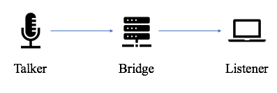
An example of a basic AVB network

IEEE 802.1AS is basically an AVB-specific profile of the IEEE 1588 standards for PTPv2. One of the editions of this standard, IEEE 802.1AS-2011, introduces gPTP (or “generalized PTP”). When used in conjunction with IEEE 1722-2011, gPTP introduces a presentation time for media data which indicates “when the rendered media data shall be presented to the viewer or listener” [25]. What I have learned from all this research is that the IEEE loves nesting new standards within other standards like a convoluted russian doll. The Stream Reservation Protocol (SRP also known as IEEE 802.1Qat) is the key that makes AVB shine from other network protocols because it allows endpoints in the network to check routes and reserve bandwidth, and SRP “checks end-to-end bandwidth availability before an A/V stream starts” [26]. This basically ensures that data won’t be sent until stream bandwidth is available and lets the endpoints decide the best route to take in the domain. So in a Dante deployment, adding additional switches daisy-chained in a network increases overall network latency the more hops that are added, and results in a need to reevaluate the network topology configuration entirely. Dante latency is set per device and depending on the size of the network, but with AVB, thanks to SRP and the QoS improvements, the bandwidth reservation gets announced through the network and latency times are kept lower even with large network deployments.

The solidity and fast communications of AVB networks have made them more common because of their ability, as the name implies, to carry audio, video, and data on the same network. The problem with all these network protocols follows the logic of Moore’s Law. If you couldn’t tell from all the revisions of IEEE standards that I have been listing, these technologies improve and get revised very quickly. Because technology is constantly improving at a blinding pace, it’s no wonder that gear manufacturing companies haven’t been able to “settle” on a common standard the way that they settled on, say, the XLR cable. This is where the newest addition to the onslaught of protocols comes in: Milan.

The standards of AVB kept developing with more improvements just like the revisions of IEEE 1588, and have led to the latest development in AVB technology called Milan. With the collaboration of some of the biggest names in the business, Milan was developed as a subset of standards within the overarching protocol of AVB. Milan includes the use of a primary and secondary redundancy scheme like that of Dante, which was not available in previous AVB networks, among other features. The key here is that Milan is open source meaning that manufacturers can develop their own implementation of Milan specific to their gear as long as it follows the outlined standards [27]. This is pretty huge if you consider how many different networking protocols are used across different pieces of gear in the audio industry. Avnu Alliance, the organization of collaborating manufacturers who developed Milan, have put together the series of specifications for Milan under the idea that any product that is released with a “Milan-ready” certification, or a badge of that nature, will be able to talk to one another over this Milan network [28].

A Note On OSC And The Future

Before we conclude our journey through the world of networking, I want to take a minute for  OSC. Open Sound Control protocol, or OSC, is an open source communications protocol that was originally designed for use with electronic music instruments but has expanded to streamlining the communications between anything from controlling synthesizers, to connecting movement trackers and software programs, to controlling virtual reality [29]. It is not an audio transport protocol, but used for device communication like MIDI (except not like MIDI because it is IP-based). I think this is a great place to end on because OSC is a great example of the power of open source technology. The versatility in OSC and its open-source platform has allowed for many programs from small to large to implement this protocol, and it is a testimony to the improvement of workflows when everyone (i.e. open-source) has the ability to input changes to make things better. We’ve spent this entire blog talking about the many different standards that have been implemented over the years to try and improve upon previous technology. Yet a gridlock of progress ensues mostly due to the fact that a standard gets made and by the time it actually gets enacted, the standard is already out of date because the technology has already surpassed that previous point in time.

So maybe it’s time for something different.

Maybe the open source nature of Milan and OSC are the way of the future because if everyone can put their heads together to try and develop specifications that are fluid and open to change as opposed to restricted by the rigidity of bureaucracy, maybe hardware will finally be able to keep up with the pace of the minds of the people using it.

Endnotes

[1] https://www.youtube.com/playlist?list=PL8dPuuaLjXtNlUrzyH5r6jN9ulIgZBpdo

[2]https://networkengineering.stackexchange.com/questions/35016/whats-the-difference-between-frame-packet-and-payload

[3] https://www.itprc.com/how-encapsulation-works-within-the-tcpip-model/

[4] https://youtu.be/9glJEQ1lNy0

[5] https://www.learncisco.net/courses/icnd-1/building-a-network/tcpip-transport-layer.html

[6] https://www.iol.unh.edu/sites/default/files/knowledgebase/1588/ptp_overview.pdf

[7] https://www.aes.org/e-lib/browse.cfm?elib=16146 (pages 1-2)

[8] https://www.nist.gov/system/files/documents/el/isd/ieee/tutorial-basic.pdf

[9] https://www.aes.org/e-lib/browse.cfm?elib=16146 (page 5)

[10] https://en.wikipedia.org/wiki/Precision_Time_Protocol

[11]https://community.cambiumnetworks.com/t5/PTP-FAQ/IEEE-1588-What-s-the-difference-between-a-Boundary-Clock-and/td-p/50392

[12]https://www.luminex.be/improve-your-timekeeping-with-ptpv2/

[13] ibid.

[14]https://www.audinate.com/company/about/history

[15]https://www.audinate.com/support/networks-and-switches

[16]https://www.luminex.be/improve-your-timekeeping-with-ptpv2/

[17]https://en.wikipedia.org/wiki/Precision_Time_Protocol

[18]https://service.shure.com/s/article/dante-and-aes-clocking-in-depth?language=en_US

[19]https://www.ravenna-network.com/app/download/13999773923/AES67%20and%20RAVENNA%20in%20a%20nutshell.pdf?t=1559740374

[20] ibid.

[21]https://www.ravenna-network.com/using-ravenna/overview

[22 ]Kreifeldt, R. (2009, July 30). AVB for Professional A/V Use [White paper]. Avnu Alliance.

[23] https://www.aes.org/e-lib/browse.cfm?elib=16147

[24] ibid.

[25] https://www.aes.org/e-lib/browse.cfm?elib=16146 (page 6)

[26] Kreifeldt, R. (2009, July 30). AVB for Professional A/V Use [White paper]. Avnu Alliance.

[27]https://avnu.org/wp-content/uploads/2014/05/Milan-Whitepaper_FINAL-1.pdf (page 7)

[28]https://avnu.org/specifications/

[29] http://opensoundcontrol.org/osc-application-areas

Resources

Audinate. (2018, July 5). Dante Certification Program – Level 3 – Module 5: IP Encapsulation [Video]. YouTube.

https://www.youtube.com/watch?v=9glJEQ1lNy0&list=PLLvRirFt63Gc6FCnGVyZrqQpp73ngToBz&index=5

Audinate. (2018, July 5). Dante Certification Program – Level 3 – Module 8: ARP [Video]. YouTube. https://www.youtube.com/watch?v=x4l8Q4JwtXQ

Audinate. (2018, July 5). Dante Certification Program – Level 3 – Module 23: Advanced Clocking [Video]. YouTube.

https://www.youtube.com/watch?v=a7Y3IYr5iMs&list=PLLvRirFt63Gc6FCnGVyZrqQpp73ngToBz&index=23

Audinate. (2019, December). The Relationship Between Dante, AES67, and SMPTE ST 2110 [White paper]. Uploaded to Scribd. Retrieved from

https://www.scribd.com/document/439524961/Audinate-Dante-Domain-Manager-Broadcast-Aes67-Smpte-2110

Audinate. (n.d.). History. https://www.audinate.com/company/about/history

Audinate. (n.d.). Networks and Switches.

https://www.audinate.com/support/networks-and-switches

Avnu Alliance. (n.d.). Avnu Alliance Test Plans and Specifications.

https://avnu.org/specifications/

Bakker, R., Cooper, A. & Kitagawa, A. (2014). An introduction to networked audio [White paper]. Yamaha Commercial Audio. Retrieved from

https://download.yamaha.com/files/tcm:39-322551

Cambium Networks Community [Mark Thomas]. (2016, February 19). IEEE 1588: What’s the difference between a Boundary Clock and Transparent Clock? [Online forum post]. https://community.cambiumnetworks.com/t5/PTP-FAQ/IEEE-1588-What-s-the-difference-between-a-Boundary-Clock-and/td-p/50392

Cisco. (n.d.) Layer 3 vs Layer 2 Switching.

https://documentation.meraki.com/MS/Layer_3_Switching/Layer_3_vs_Layer_2_Switching

Crash Course. (2020, March 19). Computer Science [Video Playlist]. YouTube. https://www.youtube.com/playlist?list=PL8dPuuaLjXtNlUrzyH5r6jN9ulIgZBpdo

Eidson, J. (2005, October 10). IEEE 1588 Standard for a Precision Clock Synchronization Protocol for Networked Measurement and Control Systems [PDF of slides]. Agilent Technologies. Retrieved from

https://www.nist.gov/system/files/documents/el/isd/ieee/tutorial-basic.pdf

Garner, G. (2010, May 28). IEEE 802.1AS and IEEE 1588 [Lecture slides]. Presented at Joint ITU-T/IEEE Workshop on The Future of Ethernet Transport, Geneva 28 May 2010. Retrieved from https://www.itu.int/dms_pub/itu-t/oth/06/38/T06380000040002PDFE.pdf

Holzinger, A. & Hildebrand, A. (2011, November). Realtime Linear Audio Distribution Over Networks A Comparison Of Layer 2 And Layer 3 Solutions Using The Example Of Ethernet AVB And RAVENNA [White paper]. Presented at the AES 44th International Conference, San Diego, CA, 2011 November 18-20. Retrieved from https://www.aes.org/e-lib/browse.cfm?elib=16147

Johns, Ian. (2017, July). Ethernet Audio. Sound On Sound. Retrieved from https://www.soundonsound.com/techniques/ethernet-audio

Kreifeldt, R. (2009, July 30). AVB for Professional A/V Use [White paper]. Avnu Alliance.

Laird, Jeff. (2012, July). PTP Background and Overview. University of New Hampshire InterOperability Laboratory. Retrieved from

https://www.iol.unh.edu/sites/default/files/knowledgebase/1588/ptp_overview.pdf

LearnCisco. (n.d.). Understanding The TCP/IP Transport Layer.

TCP vs UDP | TCP 3 Way Handshake

LearnLinux. (n.d.). ARP and the ARP table.

http://www.learnlinux.org.za/courses/build/net-admin/ch03s05.html

Luminex. (2017, June 6). PTPv2 Timing protocol in AV networks. https://www.luminex.be/improve-your-timekeeping-with-ptpv2/

Milan Avnu. (2019, November). Milan: A Networked AV System Architecture [PDF of slides].

Mullins, M. (2001, July 2). Exploring the anatomy of a data packet. TechRepublic. https://www.techrepublic.com/article/exploring-the-anatomy-of-a-data-packet/

Network Engineering [radiantshaw]. (2016, September 18). What’s the difference between Frame, Packet, and Payload? [Online forum post]. Stack Exchange.

https://networkengineering.stackexchange.com/questions/35016/whats-the-difference-between-frame-packet-and-payload

Opensoundcontrol.org. (n.d.). OSC Application Areas. Retrieved August 10, 2020 from http://opensoundcontrol.org/osc-application-areas

Perales, V. & Kaltheuner, H. (2018, June 1). Milan Whitepaper [White Paper]. Avnu Alliance. https://avnu.org/wp-content/uploads/2014/05/Milan-Whitepaper_FINAL-1.pdf

Precision Time Protocol. (n.d.). In Wikipedia. Retrieved August 10, 2020, from https://en.wikipedia.org/wiki/Precision_Time_Protocol

Presonus. (n.d.). Can Dante enabled devices exist with other AVB devices on my network? https://support.presonus.com/hc/en-us/articles/210048823-Can-Dante-enabled-devices-exist-with-other-AVB-devices-on-my-network-

Quine, A. (2008, January 27). How Encapsulation Works Within the TCP/IP Model. IT Professional’s Resource Center.

https://www.itprc.com/how-encapsulation-works-within-the-tcpip-model/

Quine, A. (2008, January 27). How The Transport Layer Works. IT Professional’s Resource Center. https://www.itprc.com/how-transport-layer-works/

RAVENNA. (n.d.). AES67 and RAVENNA In A Nutshell [White Paper]. RAVENNA. https://www.ravenna-network.com/app/download/13999773923/AES67%20and%20RAVENNA%20in%20a%20nutshell.pdf?t=1559740374

RAVENNA. (n.d.). What is RAVENNA?

https://www.ravenna-network.com/using-ravenna/overview/

Rose, B., Haighton, T. & Liu, D. (n.d.). Open Sound Control. Retrieved August 10, 2020 from https://staas.home.xs4all.nl/t/swtr/documents/wt2015_osc.pdf

Shure. (2020, March 20). Dante And AES67 Clocking In Depth. Retrieved August 10, 2020 from https://service.shure.com/s/article/dante-and-aes-clocking-in-depth?language=en_US

Weibel, H. & Heinzmann, S. (2011, November). Media Clock Synchronization Based On PTP [White Paper]. Presented at the AES 44th International Conference, San Diego, CA, 2011 November 18-20. Retrieved from https://www.aes.org/e-lib/browse.cfm?elib=16146