DFTs, FFTs, IFTs…Oh My!

The real-time analyzer (RTA) has long been a familiar tool in the audio engineer’s arsenal. Often the RTA is seen in the wild set up as a measurement microphone into an audio interface. This way the engineer can look at the frequency response of the signal received by the measurement mic. A long-time favorite application among engineers of the RTA has been for identifying frequency values for audible problems like feedback. Yet the albatross of the RTA is that it measures a single input signal with no comparison of input versus output. As one of my mentors Jamie Anderson used to say, the RTA is the “system that best correlates to our hearing”.

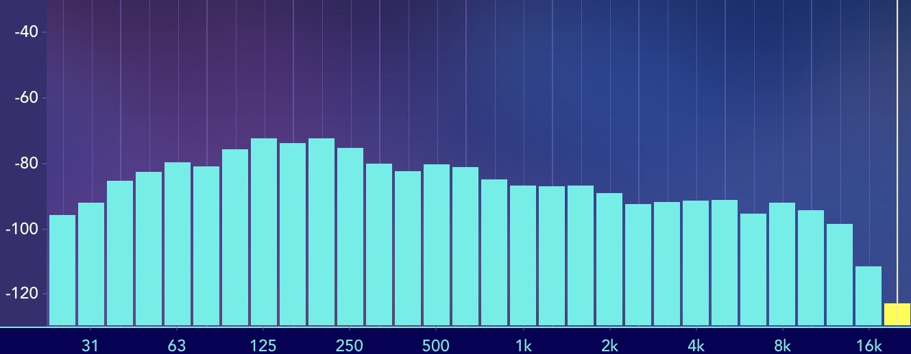
You can find a RTA in many platforms from mobile apps (Such as this screenshot from the Spectrum app) to car stereos to measurement analysis software

In one aspect, the RTA mic acts like your ears taking the input signal and displaying the frequency response. It can be viewed over a logarithmic scale similar to how we, as humans, perceive sound and loudness logarithmically. Yet even this analogy is a bit misleading because, without us realizing it, our ears themselves do a bit of signal processing by comparing what we hear to some reference in our memory. Does this kick drum sound like what we remember a kick drum to sound like? Our brain performs transfer functions with the input from our ears to tell us subjective information about what is happening in the world around us. It is through this “analog” signal processing that we process data collected from our hearing. Similarly, the RTA may seem to tell us visually about what we may be hearing, but it doesn’t tell us what the system is actually doing compared to what we put in it. This is where the value of the transfer function comes into play.

The Transfer Function and The Fourier Transform:

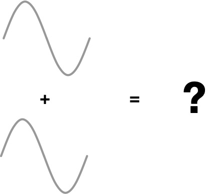
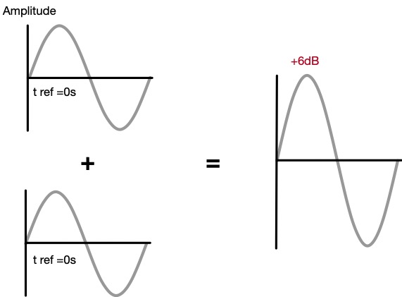
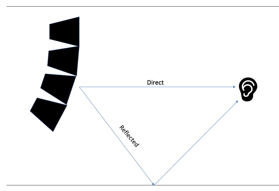
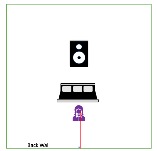
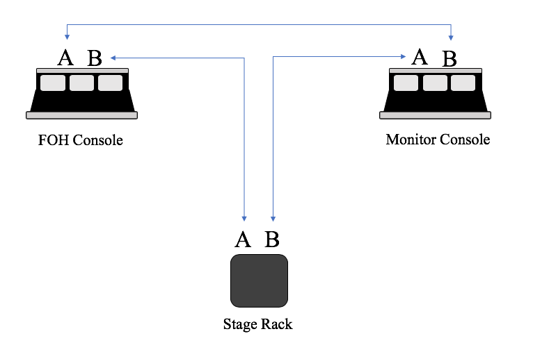
Standing at FOH in front of a loudspeaker system, you play your virtual soundcheck or favorite playback music and notice that there seems to be a change in the tonality of a certain frequency range that was not present in the original source. There could be any number of reasons why this change has occurred anywhere in the signal chain: from the computer/device playing back the content to the loudspeaker transducers reproducing it. With a single-channel analysis tool such as an RTA, one can see what is happening in the response, but not why. For example, the RTA can tell us there is a bump of +6dB at 250Hz, but just that it exists. When we take the output of a system and compare it with reference to the input of a system, then we are taking what is called a transfer function of what is happening inside that system from input to output.

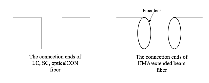
A transfer function allows for comparison of what is happening inside the system

The term “transfer function” often comes up in live sound when talking about comparing a loudspeaker system’s output with data gathered from a measurement mic versus the input signal into a processor (or output of a console, or other points picked in the signal chain). Yet a “transfer function” refers to the ratio between output and input. In fact, we can take a transfer function of all kinds of systems. For example, we can measure two electrical signals of a circuit and look at the output compared to the input. The secret to understanding how transfer functions help us in live sound lies in understanding Fourier transforms.

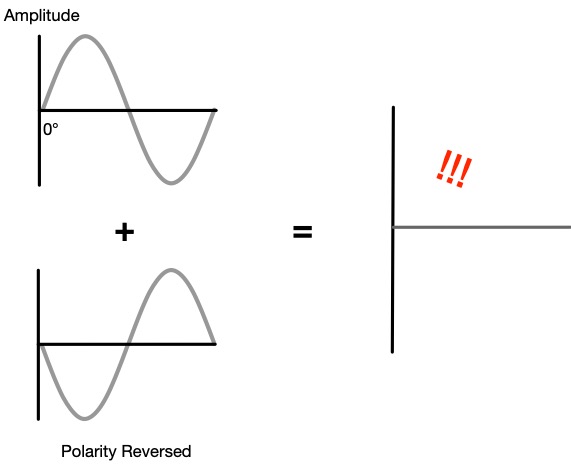
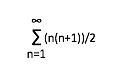
In my blog on Acoustics, I talked about how in 1807 [1], Jean-Baptiste Fourier published his discovery that complex waveforms can be broken down into their many component sine waves. Conversely, these sine waves can be combined back together to form the original complex waveform. These component sine and cosine waves comprise what is known as a Fourier series (recognize the name?). A Fourier series is a mathematical series that is composed of sine and cosine functions, as well as coefficients, that when added to infinity will replicate the original complex waveform. It’s not magic, it’s just advanced mathematics! If you really want to know the exact math behind this, check out Brilliant.org’s blog here [2]. In fact, the Fourier series was originally discovered in relation to describing the behavior of heat and thermal dynamics, not sound!

A Fourier series defines a periodic function, so one would think that since any complex wave can be broken down into its component sine and cosine waveforms over a defined period of time, then one should be able to write a Fourier series for any complex waveform…right? Well, as contributors Matt DeCross, Steve The Philosophist, and Jimin Khim point out in the Brilliant.org blog, “For arbitrary functions over the entire real line which are not necessarily periodic, no Fourier series will be everywhere convergent” [2]. This essentially means that for non-periodic functions, the Fourier series won’t always come down to a periodic, or same recurring, value. Basically, this can be extrapolated to apply to the most complex waveforms in music. The Fourier transform helps us analyze these complex waveforms.

In a PhysicsWorld video interview with Professor Carola-Bibiane Schönlieb of the University of Cambridge in the UK, she describes how the Fourier transform is a mathematical process (think multiple steps of mathematical equations here) that takes functions in the time domain and “transforms” them into the frequency domain. The important part here is that she notes how the transform function “encodes how much of every frequency, so how much of each sinusoid, of a particular frequency is present in the signal” [3]. Let’s go back to the intro of this section where we imagined sitting at FOH listening to playback and hearing a difference between the original content and the reproduced content. Conceptually, by using Fourier transforms of the output of the PA versus the input signal, one can compare how much of each frequency is in the output signal compared to the input! Before we get too excited, there are a couple of things we have to be clear about here.

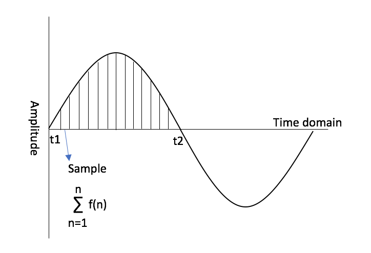
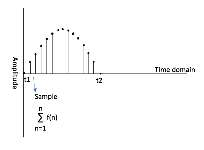
Let’s take a few conceptual steps back and briefly discuss what we really mean when we talk about “analog” versus “digital” signals. Without going into an entire blog on the topic, we can find some resolve by defining an analog signal as a continuous range of values in time, whereas digital signal processing takes discrete values of a signal sampled over some interval of time [4]. In order for us to make use of a Fourier transform in the world of digital signal processing and to transform discrete values into the frequency domain, there must be discrete values in the time domain. This seems like a rhetorical statement, but the point here is that ideally, we want our system to behave linearly so that the sum of the outputs is the same as the sum of the inputs, or rather there is some proportionality to the behavior of the output versus the input. Non-linear behavior leads to things like intermodulation distortion, which may or may not be desired in your system. It also leads to inaccurate correlations between data. In systems with linear characteristics on the output versus input in the time domain, we can perform processing with predictable, calculable responses in the frequency domain.

The DFT and The IFT

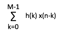
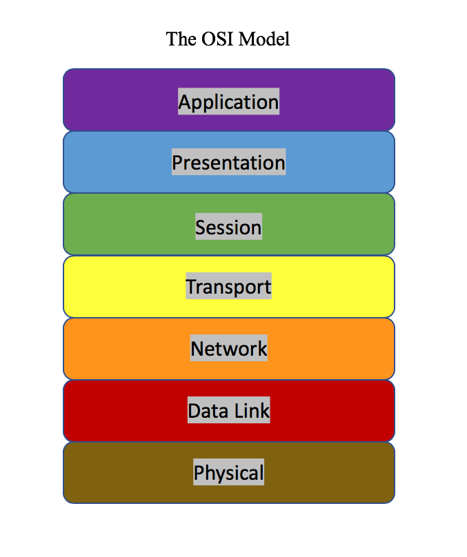
In Understanding Digital Signal Processing, Richard G. Lyons unveils that with linear time-invariant systems (so systems where the same time offset exists on the output as the input), if we know the unit impulse response (IR), we can also know the frequency response of the system using a discrete Fourier transform (DFT). Lyons defines the impulse response as “the system’s time-domain output sequence when the input is a single unity-valued sample (unit impulse) preceded and followed by zero-valued samples […]” [5]. To make a loose analogy to terms in acoustics, we can think of an impulse signal as a gunshot fired in an empty room: there is the initial amplitude of signal followed by the decay or reverberant trail of the signal heard in the room. You can imagine a unit impulse response as a version of that gunshot with no decay or reverberance and just the initial impulse, or a value like a one (as opposed to zero) over a sample of time. Lyons unveils that if we know the “unit impulse response” of the system, we can determine “the system’s output sequence for any input sequence because the output is equal to the convolution of the input sequence and the system’s impulse response […] we can find the system’s frequency response by taking the Fourier transform in the form of a discrete Fourier transform of that impulse response” [6]. If you have used a convolution reverb, you are already familiar with a similar process. The convolution reverb takes an impulse response from a beautiful cathedral or concert hall and convolves it with the input signal to create an output signal that “combines” the frequency response of the IR with the input signal. We can determine the frequency response of the system through a DFT of the impulse response, and it works both ways. By performing an inverse Fourier transform, we can take the frequency domain data and return it to the time domain and deconvolve the impulse response. The impulse response becomes the key to it all!

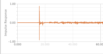
Example of an impulse response from data captured and viewed in L-Acoustics M1 software

Back when computers were less efficient, it took a lot of time to crunch these numbers for the DFT, and thus the Fast Fourier Transform (FFT) was developed to run numbers through the Fourier transform quicker. Basically, the FFT is a different algorithm (the most popular being the radix-2 FFT algorithm) that reduces the number of data points that need to be calculated [7]. Even though FFTs are still the most popular form of Fourier transform, the development of more efficient and more affordable computers allows us to crunch numbers much faster so this need for extra efficiency is less important than it used to be.

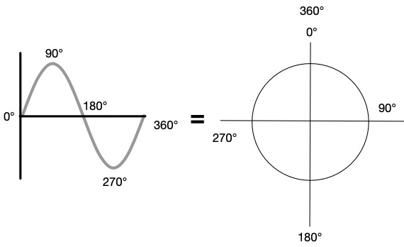
An important concept to also remember when discussing FFTs is that we are talking about digital audio and so the relationship between time and frequency becomes important in regards to frequency resolution. In my last blog “It’s Not Just a Phase,” I talk about the inverse relationship between frequency and the period of a wave. Longer wavelengths at lower frequencies take a longer period of time to complete one cycle, whereas higher frequencies with shorter wavelengths have shorter periods in time. Paul D. Henderson points out in his article, “The Fundamentals of FFT-Based Audio Measurements in SmaartLive®” that in a perfect world, one would need an infinite amount of time to reproduce the entire complex signal from a Fourier series, but this is not practical for real-world applications. Instead, we use windowing in digital signal processing to take a chunk of sampled data over a given time (called the time constant) to determine the time record of the FFT size [8]. Much like the inverse relationship between frequency and the period of a wave, the relationship between frequency resolution of the FFT is inversely proportional to the time constant. What this means is that a longer time constant results in an increase in frequency resolution, and thus lower frequencies require greater time constants. Higher frequencies require smaller time constants to get the same frequency resolution.

The first thing one may think is that longer time constants are the best way to optimize a measurement. In the days where computers were less efficient, running large FFT sizes for greater frequency resolution in low frequencies required a lot of number crunching and processing. This isn’t a problem with modern computers, but it’s also not a very efficient use of computing power. Some programs such as SMAARTv8 from Rational Acoustics offer the option to use multi-time window FFT sizes in order to optimize the time constants to provide adequate frequency resolution for different bandwidths in the frequency spectrum. For example, using a longer time constant and larger FFT size in the lower frequency range and a shorter time constant and smaller FFT size for higher frequency bandpasses.

The Importance Of The Dual-channel FFT

Now that we have a little background on what a Fourier transform is and how we got to the FFT, we can return to the topic of the transfer function mentioned earlier to discover how we can apply all this to help our situation in the FOH example earlier in this blog. With an FFT of a single source signal, we can take our impulse response and the input sequence in the time domain and convolve them to evaluate the response in the frequency domain. Let’s stop here for a second and notice that something sounds familiar. This is in fact how we can get a spectrum measurement of a single channel measurement such as that viewed in an RTA! We can see how much of each frequency is present in the original waveform, just as Carola-Bibiane Schönlieb pointed out. But what do we do if we want to see the transfer function between two signals such as the output of the PA and the input that we are feeding it? This is where we take the FFT one step further by utilizing dual-channel FFT measurements to compare the two signals and view the magnitude and phase response between them.

We can take the transfer function of our FOH example with the “output” of our system being the data gathered by measurement mic, and the “input” being the output of our console (or processor or wherever you decide to pick as the point in your signal chain). We then take a FFT of these two signals with the input being the reference and can plot out the difference in amplitude of the frequencies for different sinusoids as the magnitude response. We can also plot the offset in time between the two signals in terms of relative phase as the phase response. For more information on understanding what phase actually means, check out my last blog on phase. Many software programs utilize dual-channel FFTs to run transfer functions and show these plots so that the operator can interpret data about the system. Some examples of these programs are SMAART by Rational Acoustics, M1 by L-Acoustics, the now discontinued SIM3 by Meyer Sound, SysTune by AFMG, among others.

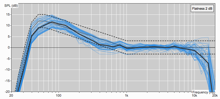
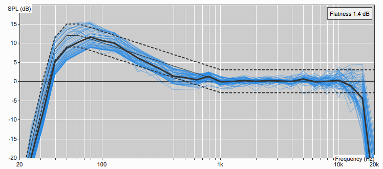
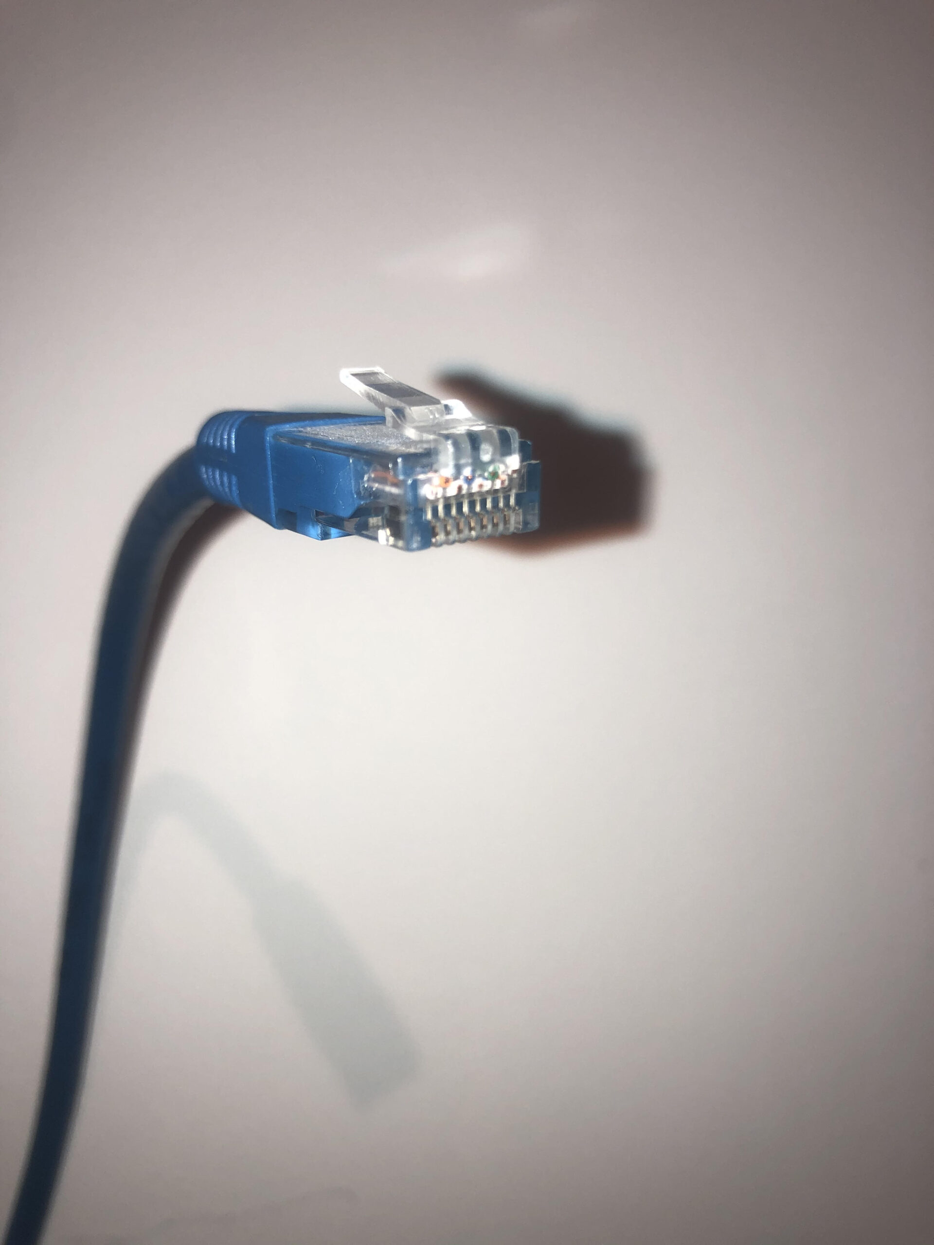
Phase (top) and magnitude (bottom) response of a loudspeaker system compared to the reference signal viewed in Rational Acoustics SMAARTv8 software

The basis of all these programs relies on the use of transfer functions to display this data. The value of these programs in aiding the engineer to troubleshoot problems in a system comes down to asking oneself what are you trying to achieve. What question are you asking of the system?

So The Question Is: What Are You Asking?

The reality of the situation is that, especially in the world of audio, and particularly in music, there is rarely a “right” or “wrong” answer. There are better solutions to solve the problem, but I would venture to say that most folks who have been on a job site or sat in the “hot seat” at a gig would argue that the answer to a problem is the one that gets the job done at the end of the day without anyone dying or getting hurt. Instead of trying to frame the discussion of the RTA versus the dual-channel FFT as a “right” or “wrong” means to an end, I want to invite the reader to ask themselves when they are troubleshooting, “What is the question I am asking? What am I trying to achieve?”. This is a point of view I learned from Jamie Anderson. If the question you are asking is “What is the frequency that correlates to what I’m hearing?” For example, in a feedback scenario, maybe the RTA is the right tool for the job. If the question is, “What is different about the output of this system versus what I put into it?” Then tools utilizing dual-channel FFTs tell you that information by comparing those signals in order to answer the question. There is no “right” or “wrong” answer, but some tools are better at answering certain questions and other tools are better at answering other questions. The beauty of the technical aspects of the audio engineering industry is that you get the opportunity to marry the creative parts of your mind with your technical knowledge and tools at your disposal. At the end of the day, all these tools are there to help you in the effort to create an experience for the audience and to realize the artists’ vision.

References:

[1] https://www.aps.org/publications/apsnews/201003/physicshistory.cfm

[2] https://brilliant.org/wiki/fourier-series/

[3] https://physicsworld.com/a/what-is-a-fourier-transform/

[4] (pg. 2) Lyons, R.G. (2011). Understanding Digital Signal Processing. 3rd ed. Prentice-Hall: Pearson Education

[5] (pg. 19) Lyons, R.G. (2011). Understanding Digital Signal Processing. 3rd ed. Prentice-Hall: Pearson Education

[6] (pg. 19) Lyons, R.G. (2011). Understanding Digital Signal Processing. 3rd ed. Prentice-Hall: Pearson Education

[7] (pg. 136) Lyons, R.G. (2011). Understanding Digital Signal Processing. 3rd ed. Prentice-Hall: Pearson Education

[8] (pg. 2) Henderson, P. (n.d.). The Fundamentals of FFT-Based Audio Measurements in SmaartLive®.

Resources:

American Physical Society. (2010, March). This Month in Physics History March 21, 1768: Birth of Jean-Baptiste Joseph Fourier. APS News. https://www.aps.org/publications/apsnews/201003/physicshistory.cfm

Cheever, E. (n.d.) Introduction to the Fourier Transform. Swarthmore College. https://lpsa.swarthmore.edu/Fourier/Xforms/FXformIntro.html

Brilliant.org. (n.d.) Fourier Series. https://brilliant.org/wiki/fourier-series/

Hardesty, L. (2012). The faster-than-fast Fourier transform. MIT News. https://news.mit.edu/2012/faster-fourier-transforms-0118

Henderson, P. (n.d.). The Fundamentals of FFT-Based Audio Measurements in SmaartLive®.

Lyons, R.G. (2011). Understanding Digital Signal Processing. 3rd ed. Prentice-Hall: Pearson Education.

PhysicsWorld. (2014) What is a Fourier transform? [Video]. https://physicsworld.com/a/what-is-a-fourier-transform/

Schönlieb, C. (n.d.). Carola-Bibiane Schönlieb. http://www.damtp.cam.ac.uk/user/cbs31/Home.html

Also check out the training available from the folks at Rational Acoustics! www.rationalacoustics.com

It’s Not Just A Phase

Understanding Phase Relationships in Constructive and Destructive Interferences

If a tree falls in the forest and nobody is there to hear it, does it make a sound? If an engineer walks between two loudspeaker systems and says it sounds “phase-y,” is there really a “phase issue”? What does that even mean?? In the world of audio, music results from the amazing amalgamation when science and art combine together. Descriptive terms often define subjective experiences whose origin can either be proven or disproven objectively using tools such as measurement devices that utilize dual-channel FFTs (Fast-Fourier Transforms). The problem that we audio engineers face when dealing with the physics of sound is that we deal with wavelengths in orders of magnitude from the size of a coin to the size of a building (see my blog on acoustics here for more info). How two different waveforms interact depends on many factors including frequency, amplitude, and phase. Not to mention what medium they are traveling through, what atmospheric conditions exist, and more…The point being is that there isn’t a one-size-fits-all answer because most of the time the answer is frequency and phase-dependent. When two correlated audio signals at the same frequency combine, do they really create 6dB of gain from summation? Well, the answer is…it depends.

Back To The Basics

Before we go any further, let’s talk about what comprises a complex waveform. In 1807, Jean-Baptiste Fourier wrote in his memoir On the Propagation of Heat in Solid Bodies [1] his theory that any complex waveform can be broken down into many component sine waves that, when reconstructed, form the original waveform. This theory would be known as a Fourier Transform [1]. The Fourier Transform forms the basis of the math that allows us to perform the signal processing in dual-channel Fast-Fourier Transforms, which in turn allow us to take data in the time domain and analyze it in the frequency domain. Without going too far down the rabbit hole of FFTs, let’s take what Jean-Baptiste Fourier has taught us about complex waveforms and know that by analyzing examples from simple sine waves, we can apply the same concepts to the behavior of more complex waveforms, but layered together to create an end result. The question then becomes what happens when you layer these simple sine waves together?

Let’s narrow our focus from complex waveforms to sine waves and first define some basic terminology such as constructive and destructive interference. When two correlated waveforms, whether it be discrete values of an electronic signal or a mathematical representation of air oscillations, combine together to create an increase in amplitude of the combining individual waveforms, it is known as constructive interference.

Figure A

When the two correlated signals combine to form a decrease in amplitude, this is called destructive interference. In the worst-case scenario, with enough offset in time or a polarity reversal of one of the individual waveforms, the waveform results in complete cancellation.

Figure B

Figure C

What’s important to note in these graphics is that both waveforms have the exact same frequency and amplitude (for the sake of this example 1000 Hz or 1kHz), but the difference is their offset in time or polarity. In Figure A, both waves start at the same time with the same amplitude so that the sum results in constructive interference which we audibly perceive as a +6dB increase in amplitude. In Figure B one wave starts at time zero while the other starts with a 0.0005s offset in time, this results in a phase offset of 180 degrees (don’t worry we will get into this more) which results in theoretical perfect cancellation of the two waveforms. Similarly in Figure C, the two waveforms start at the same time zero, but one wave has a polarity reversal where the one form starts at the crest of the wave and the other starts at the trough of the wave. This also results in a theoretical perfect cancellation, but it is important to note that a polarity reversal does not involve any offset in time. It is a physical (or electronic) “flip” of the waveform that can result from situations like having the + or – leads on a cable going to an opposite terminal on an amplifier, or pins 2 and 3 on one side of an XLR reversed compared to the other side, or the engagement of a polarity reversal switch on a console, etc. It is also important to point out that we are talking about the effects of time offset versus a polarity reversal in simple sine waves. In these cases, the destructive effects cause the same result, but as soon as we talk about complex waveforms we can definitely tell the difference between the two because there is more than one frequency involved.

So we have reviewed the basics of how waves interfere with one another, but we still haven’t explained what phase actually is. We have only talked about what happens when two waves combine and in what circumstances they will do so constructively or destructively.

In The Beginning, There Was A Circle

In order to really understand what we are talking about when we are talking about phase, we are going to dive even further back into our basic understanding of sound. Not just sound, but how we represent a wave in mathematical form. Recall that sound, in and of itself, is the oscillation of molecules (typically) air traveling through a medium and for us humans we perceive the oscillations moving the organs in our ears at rates between 20Hz to 20,000Hz (if we are lucky). We represent the patterns of this movement in mathematical form as sine waves at different frequencies (remember what Fourier said earlier about complex waveforms?). Because of the cyclical nature of these waves, i.e. the wave repeats itself after a given period, one period of the wave can be thought of as a circle unwound across a graph.

A sine wave can be thought of as an unwound circle

This concept blew my mind when I first put these two things together. The magic behind this is that many cyclical behaviors in nature from light to quantum particles can be represented through wave behavior! WOW! So now that we know that a wave is really just a circle pulled apart across the period of a given frequency (more on that to come!), we can break up a circle in terms of degrees or radians (for math and formal scientific calculations). Conversely, we can indicate what position at a particular point along that waveform is in terms of degrees or radians along the circle. This is the phase at that given position. In the analog world, we talk about phase in relation to time because it took some amount of time, however small, for the waveform to get to that particular position. So how do we figure out what the phase is at a given time for a given frequency sine wave? Time for some more math!

Three Important Formulas in Sound

If you can imprint in your brain three formulas that can be applied to sound for the rest of your life, I highly recommend remembering these three (though we will only really go into two in this blog):

1/T=f or 1/f=T

1/period of a wave in seconds (s) = frequency (in cycles per second or Hertz (Hz))

1/frequency of a wave (Hz) = period of a wave (in seconds)

λ =c/f

wavelength (feet or meters) = speed of sound (feet per second ft/s or meters per second m/s) / frequency (Hz)

**must use the same units of distance on both sides of the equation!! (feet or meters)**

V=IR (Ohm’s Law (DC version))

Voltage (Volts) =Current (Amperes) x Resistance (Ohms)

The first equation is very important because it shows the reciprocal relationship between the period of a wave (the overall duration in time for one cycle to complete) to the frequency of the wave (in cycles per second or Hertz). Let’s go back to the example from before of the 1,000Hz sine wave. Using one form of the first equation T=1/f we find that for a 1,000Hz sine wave:

1/1,000 Hz = 0.001 s

The period of a 1,000Hz sine wave is 0.001s or 1 millisecond (1ms). We can visualize this as the amount of time it takes to complete one full cycle and travel from 0 to 360 degrees around the 1,000Hz circle as 1ms or 0.001s.

1,000Hz sine wave with a period of 1ms

The thing is, in most scenarios, phase doesn’t have much meaning to us unless it’s in relation to something else. Time doesn’t have much meaning to us unless it’s in relation to another value. For example, we aren’t late for a meeting unless we had to be there at noon and it is now 2:00 pm. If the meeting had no time reference, would we ever be late? Similarly, a signal by itself can start at any given position in-phase/time and it’s just the same signal…later in time…But if you combine two signals, one starting at one time and the other offset by some value in time, now we start to have some interaction.

Since we now understand phase as a value for a position in time along the period of a waveform, we can do a little math magic to figure out what the phase offset is based on the time offset between two waveforms. Let’s take our 1,000Hz waveform and now copy it and add the two together, except this time one of the waveforms is offset by 0.0005s or 0.5ms. If we take the ratio of the time offset divided by the period of the 1,000Hz waveform (0.001s or 1ms) and multiply that by 360 degrees, we get the phase offset between the two signals in degrees.

(360 degrees )*((time offset in seconds / period of wave in seconds))

(360)*((0.0005)(0.001))=180 degrees

That means that when two copies of the same correlated 1,000Hz signals are offset by 0.5ms they are offset by 180 degrees! If you combined these two at equal amplitude you would get destructive interference resulting in near-perfect cancellation! Knowing the frequency of interacting waves is only part of the picture. We can see that the phase relationship between correlated signals is equally important to understanding whether the interference will be constructive or destructive. It should be noted here that in all these examples we are talking about combining correlated signals of equal amplitude. If we have an amplitude or level offset between the signals, that will affect the summation as well! So how do we know whether a phase offset or offset in time will be destructive or constructive? Is it arbitrary? The answer is: it depends on the frequency!

Understanding Phase In Relation to Frequency

Remembering our 1,000Hz sine wave has a period of 1ms based on using the formula for the reciprocal relationship between frequency and period, let’s find the period of a 100Hz waveform:

1/f=T

1/100=0.01s or 10ms

That means the period of a 100Hz wave is ten times longer than the period of a 1,000Hz wave! A time offset between two copies of the same frequency wave at equal amplitude will have phase offsets dependent on their frequency because of their different periods. For example, the 0.5ms offset between two 1,000 Hz waveforms results in a 180 degree offset, but if we do the math for the same offset in time between two 100Hz waves,

(360 degrees)(0.0005s/0.01s)=18 degrees

That’s only an offset of 18 degrees! Will an 18 degree offset of two correlated sine waves at 100Hz have a constructive or destructive effect? (Remember for the sake of simplicity we are assuming equal amplitude for these examples). In order to understand this, let’s look back at a basic drawing of a sine wave:

Figure D

So here is the really cool part: much like we can use a sine wave or a circle to represent the cyclical nature of the period of a wave, we can also use a sine wave to describe the relationship between identical waveforms as well! Or rather we can use a sine wave/circle to describe the phase relationship between the two waves as an offset between the two waveforms because the effects are also cyclical in nature! We just went through the math of how different time offsets equate to a different phase relationship depending on frequency, so if you were to look at the effects of a time offset across a spectrum of frequencies, you would see a cyclical waveform of that phase response itself as it changes depending on the frequency! It’s like a sine wave inception!!

In Figure D we see the markings for phase along the waveform or unwrapped circle as we learned earlier. We have also learned that these positions in time will change depending on the period/frequency of the waveform. Visually we can see as you approach 90 degrees on the sine wave, the slope of the wave increases up until roughly the 60-degree point where it begins to “flatten” out. This means if we were interpreting this as the phase response between two correlated signals, the resultant wave would still be increasing in amplitude. The summation of two identical, correlated waveforms at this offset will still result in addition. From +6dB when there is 0 degree offset since the two waveforms begin at the same time, up to 3dB at 90 degrees. Yet after 90 degrees, the slope begins to decrease, indicating that when we combine two identical waveforms with an offset in this range we begin losing summation and enter destructive interference until we reach 180 degrees, which results in theoretical perfect cancellation. As we continue our journey along the period of this waveform, we continue with destructive interference to a lessening degree until the trough of the waveform “flattens” out again at 270 degrees where we again have reached +3dB summation. After 270 degrees we increase in amplitude until we reach 360 degrees at which point we have made it all the way around the circle and the entire period of the waveform to 6dB of summation again. Merlijn Van Veen has a great graphic of the “wheel of phase” on his website that offers a visual representation of the relative gain (in decibels) between two identical, correlated signals as indicated by their phase relationship [2].

What this means is that whether two correlated signals will combine to form a destructive or constructive resultant waveform will depend on their frequency, amplitude, and phase relationship to one another. It’s easy to extrapolate that as you start talking about complex waveforms interacting, you are managing multiple frequencies at different amplitudes so describing the phase relationships between the interactions becomes more and more convoluted.

And Now Comb Filters

So now that we have come back from this world of mathematical representations of real-world behaviors, how can we actually apply this to the real world? Recall from the beginning of this blog the example of the engineer walking between two loudspeakers and declaring it to sound “phase-y”. Here is where we can finally understand what the engineer is hearing by using our new understanding of what phase actually means to describe the audible peaks and dips of the comb filter. A comb filter results from the combination of two wide-spectrum signals with some offset in the time domain. In fact, any change in level or phase relationship between the two correlated signals will affect the severity of the comb filter. Let’s imagine that the engineer is listening at a position equidistant from the two loudspeakers that are spaced equal distance apart from their acoustic centers and both have fairly wide dispersion patterns. For the sake of relative simplicity, we will make them directional point sources with a pattern wide enough to fully overlap each other. Let’s then imagine that both loudspeakers are playing the same identical broadband pink noise signal to both loudspeakers. With both loudspeakers playing identical signals at identical time, the engineer should hear an additive 6dB of summation from the two signals adding together. If one of the speakers gets pushed back roughly 1.125ft or gets 1ms of time delay added electronically via the DSP, the engineer will hear the resultant comb filter at the listening position. There will be a 1,000Hz spacing between nulls of this comb filter. We can figure that out using two of our handy physics equations from earlier. For the time offset of 1ms:

f=1/T so 1/0.001s=1,000Hz

And if we physically pushed back the speaker about 1ft, we can use the formula for wavelength to find the frequency:

Wavelength = speed of sound / frequency

or in this case, by doing some algebra we can rewrite that as:

Frequency = speed of sound / wavelength

The speed of sound at “average sea level”, which is roughly 1 atmosphere or 101.3 kiloPascals [3]), at 68 degrees Fahrenheit (20 degrees Celsius), and at 0% humidity is approximately 343 meters per second or approximately 1,125 feet per second [4] (see more about this in my blog on Acoustics). If we calculate this using the speed of sound in ft/s since our measurement of the displacement is in feet, we again get the resultant comb filter spacing of 1,000Hz:

1,125 ft/s / 1.125ft = 1,000Hz

Both equations allow us to predict or explain anomalies that we hear. These equations allow us to understand how to calculate the general behavior of comb filters! Now we can take this one step further by talking about subwoofer spacing.

There is a common trope in live sound of spacing subs within a “quarter-wavelength apart”. Using our knowledge of how the phase relationship between two correlated waveforms will be frequency-dependent, we can understand on a basic level (without taking into account room acoustics and other complex acoustical calculations) how if you take a critical frequency say of 60Hz and use that as your “frequency of interest” if you stay within 60 degrees of time offset between the two subwoofers, they will still result in summation to some degree at that frequency.

The truth is that understanding the interactions of complex waveforms involves not just doing these calculations based on one frequency of interest. We are dealing with complex waveforms composed of many different frequencies all in orders of magnitude different from one another with behavior that changes depending on what frequency bandpass you are talking about. Not to mention also including the interactions of room acoustics, atmospheric conditions, and other external factors. There is no one-size-fits-all solution, but by breaking down complex waveforms into their component sine waves and using the advancements in technology and analysis tools to crunch the numbers for us, we can use all the tools at our disposal to see the bigger picture of what’s happening when two waveforms interact.

Endnotes:

[1] https://www.aps.org/publications/apsnews/201003/physicshistory.cfm

[2] https://www.merlijnvanveen.nl/en/study-hall/169-displacement-is-key

[3] (pg. 345) Giancoli, D.C. (2009). Physics for Scientists & Engineers with Modern Physics. Pearson Prentice Hall.

[4] http://www.sengpielaudio.com/calculator-airpressure.htm

Resources:

Everest, F.A. & Pohlmann, K. (2015). Master Handbook of Acoustics. 6th ed. McGraw-Hill Education.

Lyons, R.G. (2011). Understanding Digital Signal Processing. 3rd ed. Prentice-Hall: Pearson Education.

van Veen, M. (2019). Displacement is Key. Merlijn van Veen. https://www.merlijnvanveen.nl/en/study-hall/169-displacement-is-key

Depression, Anxiety, and Hope from a Roadie In The Age of Covid

Dear Everyone, you are not alone.

**TRIGGER WARNING: This blog contains personal content surrounding issues of mental health including depression and anxiety, and the Covid-19 pandemic. Reader discretion is advised.**

The alarm on my phone went off at 6:30 a.m.

I rolled out of my bunk, carefully trying to make as little noise as possible as I gathered my backpack, clothes, and tool bag before exiting the bus.

The morning air felt cool against my face as I looked around me trying to orient myself in the direction of the loading dock to the arena. Were we in New York? Ohio? Pennsylvania? In the morning before coffee, those details were difficult to remember.

Passed the elephant door, the arena sprawled out before me, empty and suspensefully silent. I looked up with a mixed sense of awe and critical analysis as I noted the three tiers of the arena, the red seats forming distinct geometrical shapes between each section. As I made my way out to the middle of the deceivingly large room, I looked toward the ground in hopes of finding that tell-tale button marking the middle of the room, if I was lucky.

As I set up my tripod, I heard the footsteps of the rigging team as they began stretching out their yellow measuring tapes across the cement floor. The clapping of their feet echoed in the room and soon the sound of their voices calling out distances joined the chorus in the reverb tails.

I turned on my laser and pulled out my notepad, the pen tucked in my hair as I aimed for the first measurement.

Then I woke up.

Up above me, all I could see was the white air-tile of the basement ceiling while the mini-fridge hummed in the corner of the room.

For a few seconds, or maybe it was a full minute, I had absolutely no idea where I was.

I wanted to scream.

I lay in bed for what could have been 15 minutes or an hour, telling myself I had to get out of bed. I couldn’t just lay here. I had to do something. Get up. Get UP.

Eventually, I made my way upstairs and put on a pot of water for coffee. When I opened my phone and opened Facebook, I saw a status update from a friend about a friend of a friend who had passed away. My heart sank. I remembered doing a load-in with that person. Years ago, at a corporate event in another city, in another lifetime. They didn’t post details on what had happened to them. Frankly, it wasn’t anyone’s business, but the family and those closest to them. Yet my heart felt heavy.

Six months ago, or maybe more, time had ceased to have any tangible meaning at this point, I had been sitting in a restaurant in Northern California when the artists told the whole tour that we were all going home. Tomorrow. Like a series of ill-fated dominoes, events were canceling one-by-one across the country and across the world. Before I knew it, I was back in my storage unit at my best friend’s house, trying to shove aside the boxes I had packed up 4 or 5 months earlier to make room for an inflatable mattress so I had somewhere to sleep. I hadn’t really expected to be “home” yet so I hadn’t really come up with a plan as to what I was going to do.

Maybe I’ll go camping for the next month or so. Try to get some time to think. I loved nature and being out in the trees always made me feel better about everything, so maybe that was the thing to do. Every day I looked at the local newspaper’s report of the number of Covid-19 cases in California. It started out in the double digits. The next day it was in the triple digits. Then it grew again. And again. Every day the numbers grew bigger and notices of business closing and areas being restricted filled the pages and notifications across the Internet.

Fast-forward and the next thing I knew, I was packing all my possessions into a U-Haul trailer and driving across the country to be with my sister in Illinois. She had my baby niece a little over a year ago, so I figured the best use of my time would be to spend time with my family while I could.

I was somewhere driving across Kansas when the reality of what was happening hit me. As someone who loved making lists and planning out everything from their packing lists to their hopes and dreams in life, I—for once—literally had no idea what I was doing. This seemed like the best idea I could think of at the time.

Fast-forward and I was sitting on the phone in the basement of my sister’s house in the room she had graciously fabricated for me out of sectioned-off tapestries. I looked at the timestamp on my phone for how long I had been on hold with the Unemployment Office. Two hours and thirty minutes. It took twenty calls in a row to try and get through to someone at the California Employment Development Department. At the three-hour mark, the line disconnected. I just looked down at my phone.

I remember one Christmas when I was with my dad’s side of the family at dinner, I tried to explain what I do to them.

“So you are a DJ, then?” my aunt asked enthusiastically, believing that she had finally gotten it right.

“No,” I said.

“Do you play with the band?” my uncle asked.

“No, I’m the person who tries to make sure everyone in the audience can hear the band,” I tried to laugh.

Everyone laughed that sort of half-laugh when you try to pretend you get the joke, but you don’t actually get it.

Across my social media feeds, friends, colleagues, acquaintances, and everyone in between, were all sharing updates of how they had to get “real jobs”, how they couldn’t get through to unemployment or their state had completely failed to get them any unemployment at all, how they were angry, desperate, and how they needed to feed their families. Leaders in the industry grew from the motivation of trying to speak out on behalf of the live events industry to the government, pleading for financial relief for businesses, venues, individuals, and more, and my feeds flooded with initiatives and campaigns for awareness of the plight of the live events industry.

Yet when I talked to people who were not in the industry, they seemed to have no idea that the live events sector had been affected at all. Worse yet, I realized more and more that so few people had any idea of what people in the live events industry actually do. Organizations struggled to get news channels to do exposés on the subject, and perhaps it was because there were so many people across every sector of every industry that were struggling. In one conversation with a friend, I had explained that there were nearly 100 people on a tour that I had worked on between the production, tech crew, artist’s tech crew, everyone. They couldn’t believe so many people were working behind the scenes at one concert.

Yet the more I talked about my job and the more time that passed, the more I felt like I was talking about a dream. This fear grew inside me that there was no end in sight to all this and the stories started to repeat themselves and it started to feel like these were stories of what had been, not what was. It was becoming increasingly difficult to concentrate when talking to people about “regular” things in our daily lives because it was not work. Talking about the weather was not talking about rigging plots or truckloads, so my brain just refused to focus on it. Yet I couldn’t stop thinking about the industry: watching webinars, learning new things because I just wanted so desperately to go back to my career that I fabricated schedules and deadlines around other obligations to feel like work was still there.

Then the thought that underpinned all this rose up like a monster from the sea:

Who am I without my job?

I read an article Dave Grohl wrote [1] about performing and playing music on-stage for people, how there was nothing like that feeling in the whole world. I think he hit on something that, in effect, is really indescribable to anyone who has not worked in the live events world. There was a feeling unlike any other of standing in a room with tens of thousands of people screaming at deafening levels. There was a feeling unlike any other of standing alone in a room listening to a PA and crafting it to sound the way you wanted it to. There was a feeling unlike any other of hearing motors running in the morning while pulling a snake across an arena floor. There was a feeling unlike any other of complete, utter exhaustion riding a bus in the morning to the next load-in after doing 4, 5, 6, however many gigs in a row. I tried to explain these feelings to my friends and family who listened with compassion, but I couldn’t help but feel that sometimes they were just pretending to get the joke.

Days, weeks, months floated by and the more time passed, the more I felt like I was floating in a dream. This was a bad dream that I would wake up from. It had to be. Then when I came to reality and realized that this was not a dream, that this was where I was in my life now, it felt like my brain and the entire fabric of my being was splitting in two. It was not unbeknownst to me how fortunate I was with my sister taking me in. Every morning I tried to say 5 things I was grateful for to keep my spirits up and my sister was always one of them.

The painful irony was that I had stopped going to therapy in January 2020 because I felt I had gotten to an OK point in my life where I was good for now. I had gotten where I needed to for the time being and I could shelve all the other stuff for now until I had time to address them. Then suddenly I had all the time in the world and while shut down in quarantine, all those things in my brain I told myself I would deal with later…Well, now I had no other choice than to deal with them, and really this all intersected with the question at hand of who was I without my job.

And I don’t think I was alone

The thing people don’t tell you about working in the industry is the social toll it takes on your life and soul. The things you give up and the parts of yourself you give up to make it a full-time gig. Yet there is this mentality of toughing it through because there are 3,000 other people waiting in line to take your spot and if you falter for even just one step, you could be gone and replaced just as easily. Organizations focusing on mental health in the industry started to arise from the pandemic because, in fact, it wasn’t just me. There are many people who struggle to find that balance of life and work let alone when there is a global health crisis at hand. All this should make one feel less alone, and to some extent it does. The truth is that the journey towards finding yourself is, as you would imagine, something each person has to do for themself. And my reality was that despite all the sacrifices needed for this job, all I wanted to do was run back to it as fast as I could.

Without my work, it felt like a huge hole was missing from my entire being. That sense of being in a dream pervaded my every waking moment and even in my dreams, I dreamt of work to the point where I had to take sleeping aids just so I would stop thinking about it in my dreams too. I found myself at this strange place in my life where I reunited myself with hobbies that I previously cast aside for touring life and trying to appreciate what happiness they could offer. More webinars and industry discussions popped up about “pivoting” into new industries or fields and in some of these, you could physically see the pain in the interviewees’ faces as they tried to discuss how they had made their way in another field.

One day I was playing with my baby niece and I told her we had to stop playing to go do something, but we would come back to playing later. She just looked at me in utter bewilderment and said, “No! No! No!” Then I remembered that small children have no concept of “now” versus “later”. Everything literally is in the “now” for them. It struck me as something very profound that my niece lived completely in the moment. Everything was a move from one activity to the next, always moving forward. So with much effort and pushback against every fiber of my future-thinking self, I just stopped trying to think of anything further than the next day ahead of me. Just move one foot in front of the other and be grateful every day that I am here in what’s happening at this moment.

Now with the vaccination programs here in the United States and the rumblings of movement trickling across the grapevine, it feels like for the first time in more than a year that there is hope on the horizon. There is a part of me that is so desperate for it to be true and part of me that is suspiciously wary of it being true. Like seeing the carrot on the ground, but being very aware of the fact there is a string attached to it that can easily pull the carrot away from you once more.

There is a hard road ahead and a trepidatious one, at that. Yet after months and months of complete uncertainty, there is something to be said about having hope that things will return to a new type of “normal”. Because “normal” would imply that we would return to how things were before 2020. I believe that there is good change and reflection that came in the pause of the pandemic that we should not revert back from: a collective reflection on who we are, whether we wanted to address it to ourselves or not.

What will happen from this point moving forward is anyone’s gamble, but I always like to think that growth doesn’t come from being comfortable. So with one foot in front of the other, we move forward into this next phase of time. And like another phrase that seems to come up over and over again, “Well, we will cross that bridge when we come to it.”

References:

[1]https://www.theatlantic.com/culture/archive/2020/05/dave-grohl-irreplaceable-thrill-rock-show/611113/

What Is a FIR Filter?

The use of FIR filters (or finite impulse response filters) has grown in popularity in the live sound world as digital signal processing (DSP) for loudspeakers becomes more and more sophisticated. While not a new technology in itself, these filters provide a powerful tool in system optimization due to their linear phase properties. But what exactly do we mean by “finite impulse response” and how do these filters work? In order to understand digital signal processing better we are going to need to take a step back into our understanding of mathematics and levels of abstraction.

A (Very) Brief Intro To DSP

One of the reasons I find mathematics so awesome is because we are able to take values in the real or imaginary world and represent them either symbolically or as a variable in order to analyze them. We can use the number “2” to represent two physical oranges or apples. Similarly, we can take it up another level of abstraction by saying we have “x” amount of oranges or apples to represent a variable amount of said item. Let’s say we wanted to describe an increasing amount of apples where for every new index of apples, we add the sum of the previous number of apples. We can write this as an arithmetic series for all positive integer number “n” of apples as:

Where for each index of apples starting at 1, 2, 3, 4…etc onto infinity we have the current index value n plus the sum of all the values before it. Ok, you might be asking yourself why we are talking about apples when we are supposed to be talking about FIR filters. Well, the reason is that digital signal processing can be represented using this series notation and it makes it a lot easier than writing out the value for every single input into a filter. If we were to sample a sine wave like the one below, we could express the total number of samples over the period from t1 to t2 as the sum of all the samples over that given period.

In fact, as Lyons points out in Understanding Digital Signal Processing (2011) we can express the discrete-time sequence for a given sine-wave at frequency f (in Hertz) at a given time t (in seconds) with the function f(n) = This equation allows us to translate each value of the sine wave, for example, voltage in an electric signal, for a discrete moment in time into an integer value that can be plotted in digital form.

What our brain wants to do is draw lines in between these values to create a continuous waveform so it looks like the original continuous sine wave that we sampled. In fact, this is not possible because each of these integers are discrete values and thus must be seen separately as compared to an analog, continuous signal. Now, what if the waveform that we sampled wasn’t a perfect sine wave, but instead had peaks and transient values? The nature of FIR filters has the ability to “smooth out” these stray values with linear phase properties.

How It Works

The finite impulse response filter gets its name because the same number, or finite, input values you get going into the filter, you get coming out the output. In Understanding Digital Signal Processing, Lyons uses a great analogy of how FIR filters average out summations like averaging the number of cars crossing over a bridge [2]. If you counted the number of cars going over a bridge every minute and then took an average over the last five minutes of the total number of cars, this averaging has the effect of smoothing out the outlying higher or lower number of vehicles to create a more steady average over time. FIR filters function similarly by taking each input sample and multiplying it by the filter’s coefficients and then summing them at the filter’s output. Lyons points out how this can be described as a series which illustrates the convolution equation for a general “M-tap FIR filter” [3]:

While this may look scary at first, remember from the discussion at the beginning of this blog that mathematical symbols package concepts into something more succinct for us to analyze. What this series is saying is that for every sample value x whose index value is n-k, k being some integer greater than zero, we multiply its value times the coefficient h(k) and sum the values for the number of taps in the filter (M-1). So here’s where things start to get interesting: the filter coefficients h(k) are the FIR filter’s impulse response. Without going too far down the rabbit hole in discussing convolution and different types of FIR windows for filter design, let’s jump into the phase properties of these filters then focus on their applications.

The major advantage of the FIR filter compared to other filters such as the IIR (or infinite impulse response) filter lies in the symmetrical nature of the delay introduced into the signal that doesn’t introduce phase shift into the output of the system. As Lyons points out this relates to the group delay of the system:

When the group delay is constant, as it is over the passband of all FIR filters having symmetrical coefficients, all frequency components of the filter input signal are delayed by an equal amount of time […] before they reach the filter’s output. This means that no phase distortion is induced in the filter’s desired output signal […] [4]

It is well known that phase shift, especially at different frequency ranges, can cause detrimental constructive and/or destructive effects between two signals. Having a filter at your disposal that allows gain and attenuation without introducing phase shift has significant advantages especially when used as a way of optimizing frequency response between zones of loudspeaker cabinets in line arrays. So now that we have talked about what a FIR filter is and its benefits, let’s discuss a case for the application of FIR filters.

Applications of FIR filters

Before sophisticated DSP and processors were so readily available, a common tactic of handling multiway sound systems, particularly line arrays, with problematic high-frequencies was to go up to the amplifier of the offending zone of boxes and physically turn down the amplifier running the HF drivers. I’m not going to argue against doing what you have to do to save people’s ears in dire situations, but the problem with this method is that when you change the gain of the amplifier for the HF in a multiway loudspeaker, you effectively change the crossover point as well. One of our goals in optimizing a sound system is to maintain the isophasic response of the array throughout all the elements and zones of the system. By using FIR filters to adjust the frequency response of a system, we can make adjustments and “smooth out” the summation effects of the interelement angles between loudspeaker cabinets without introducing phase shift in-between zones of our line array.

Remember the example Lyons gave comparing the averaging effects of FIR filters to averaging the number of cars crossing a bridge? Now instead of cars, imagine we are trying to “average” out the outlier values for a given frequency band in the high-frequency range of different zones in our line array. These variances are due to the summation effects dependent on the interelement angles between cabinets. Figure A depicts a 16 box large-format line array with only optimized interelement angles between boxes using L-Acoustics’ loudspeaker prediction software Soundvision.

Figure A

Each blue line represents a measurement of the frequency response along the coverage area of the array. Notice the high amount of variance in frequency response particularly above 8kHz between the boxes across the target audience area for each loudspeaker. Now when we use FIR filtering available in the amplifier controllers and implemented via Network Manager to smooth out these variances like in the car analogy, we get a smoother response closer to the target curve above 8kHz as seen in Figure B.

Figure B

In this example, FIR filtering allows us to essentially apply EQ to individual zones of boxes within the array without introducing a relative phase shift that would break the isophasic response of the entire array.

Unfortunately, there is still no such thing as a free lunch. What you win in phase coherence, you pay for in propagation time. That is why, sadly, FIR filters aren’t very practical for lower frequency ranges in live sound because the amount of introduced delay at those frequency ranges would not be practical in real-time applications.

Conclusion

By taking discrete samples of a signal in time and representing it with a series expressions, we are able to define filters in digital signal processing as manipulations of a function. Finite impulse response filters with symmetric coefficients are able to smooth out variances in the input signal due to the averaging nature of the filter’s summation. The added advantage here is that this happens without introducing phase distortion, which makes the FIR filter a handy tool for optimizing zones of loudspeaker cabinets within a line array. Today, most professional loudspeaker manufacturers employ FIR filters to some degree in processing their point source, constant curvature, and variable curvature arrays. Whether the use of these filters creates a smoother sounding frequency response is up to the user to decide.

Endnotes:

[1] (pg. 2) Lyons, R.G. (2011). Understanding Digital Signal Processing. 3rd ed. Prentice-Hall: Pearson Education.

[2] (pg. 170) Lyons, R.G. (2011). Understanding Digital Signal Processing. 3rd ed. Prentice-Hall: Pearson Education.

[3] (pg. 176) Lyons, R.G. (2011). Understanding Digital Signal Processing. 3rd ed. Prentice-Hall: Pearson Education.

[4] (pg. 211) Lyons, R.G. (2011). Understanding Digital Signal Processing. 3rd ed. Prentice-Hall: Pearson Education.

Resources:

John. M. (n.d.) Audio FIR Filtering: A Guide to Fundamental FIR Filter Concepts & Applications in Loudspeakers. Eclipse Audio. https://eclipseaudio.com/fir-filter-guide/

Lyons, R.G. (2011). Understanding Digital Signal Processing. 3rd ed. Prentice-Hall: Pearson Education.

One Size Does Not Fit All in Acoustics

Have you ever stood outside when it has been snowing and noticed that it feels “quieter” than normal? Have you ever heard your sibling or housemate play music or talk in the room next to you and hear only the lower frequency content on the other side of the wall? People are better at perceptually understanding acoustics than we give ourselves credit for. In fact our hearing and our ability to perceive where a sound is coming from is important to our survival because we need to be able to tell if danger is approaching. Without necessarily thinking about it, we get a lot of information about the world around us through localization cues gathered from the time offsets between direct and reflected sounds arriving at our ears that our brain performs quick analysis on compared to our visual cues.

Enter the entire world of psychoacoustics

Whenever I walk into a music venue during a morning walk-through, I try to bring my attention to the space around me: What am I hearing? How am I hearing it? How does that compare to the visual data I’m gathering about my surroundings? This clandestine, subjective information gathering is important to reality check the data collected during the formal, objective measurement processes of systems tunings. People spend entire lifetimes researching the field of acoustics, so instead of trying to give a “crash course” in acoustics, we are going to talk about some concepts to get you interested in the behavior that you have already been spending your whole life learning from an experiential perspective without realizing it. I hope that by the end of reading this you will realize that the interactions of signals in the audible human hearing range are complex because the perspective changes depending on the relationships of frequency, wavelength, and phase between the signals.

The Magnitudes of Wavelength

Before we head down this rabbit hole, I want to point out one of the biggest “Eureka!” moments I had in my audio education was when I truly understood what Jean-Baptiste Fourier discovered in 1807 [1] regarding the nature of complex waveforms. Jean-Baptiste Fourier discovered that a complex waveform can be “broken down” into its many component waves that when recombined create the original complex waveform. For example, this means that a complex waveform, say the sound of a human singing, can be broken down into the many composite sine waves that add together to create the complex original waveform of the singer. I like to conceptualize the behavior of sound under the philosophical framework of Fourier’s discoveries. Instead of being overwhelmed by the complexities as you go further down the rabbit hole, I like to think that the more that I learn, the more the complex waveform gets broken into its component sine waves.

Conceptualizing sound field behavior is frequency-dependent

One of the most fundamental quandaries about analyzing the behavior of sound propagation is due to the fact that the wavelengths that we work with in the audible frequency range vary in orders of magnitude. We generally understand the audible frequency range of human hearing to be 20 cycles per second (Hertz) -20,000 cycles per second (20 kilohertz), which varies with age and other factors such as hearing damage. Now recall the basic formula for determining wavelength at a given frequency:

Wavelength (in feet or meters) = speed of sound (feet or meters) / frequency (Hertz) **must use same units for wavelength and speed of sound i.e. meters and meters per second**

So let’s look at some numbers here given specific parameters of the speed of sound since we know that the speed of sound varies due to factors such as altitude, temperature, and humidity. The speed of sound at “average sea level”, which is roughly 1 atmosphere or 101.3 kiloPascals [2]), at 68 degrees Fahrenheit (20 degrees Celsius), and at 0% humidity is approximately 343 meters per second or approximately 1,125 feet per second [3]. There is a great calculator online at sengpielaudio.com if you don’t want to have to manually calculate this [3]. So if we use the formula above to calculate the wavelength for 20 Hz and 20kHz with this value for the speed of sound we get (we will use Imperial units because I live in the United States):

Wavelength of 20 Hz= 1,125 ft/s / 20 Hz = 56.25 feet

Wavelength of 20 kHz or 20,000 Hertz = 1,125 ft/s / 20,000 Hz = 0.0563 feet or 0.675 inches

This means that we are dealing with wavelengths that range from roughly the size of a penny to the size of a building. We see this in a different way as we move up in octaves along the audible range from 20 Hz to 20 kHz because as we increase frequency, the number of frequencies per octave band increases logarithmically.

32 Hz-63 Hz

63-125 Hz

125-250 Hz

250-500 Hz

500-1000 Hz

1000-2000 Hz

2000-4000 Hz

4000-8000 Hz

8000-16000 Hz

Look familiar??

Unfortunately, what this ends up meaning to us sound engineers is that there is no “catch-all” way of modeling the behavior of sound that can be applied to the entire audible frequency spectrum. It means that the size of objects and surfaces obstructing or interacting with sound may or may not create issues depending on its size in relation to the frequency under scrutiny.

For example, take the practice of placing a measurement mic on top of a flat board to gather what is known as a “ground plane” measurement. For example, placing the mic on top of a board, and putting the board on top of seats in a theater. This is a tactic I use primarily in highly reflective room environments to take measurements of a loudspeaker system in order to observe the system behavior without the degradation from the reflections in the room. Usually, because I don’t have control over changing the acoustics of the room itself (see using in-house, pre-installed PAs in a venue). The caveat to this method is that if you use a board, the board has to be at least a wavelength at the lowest frequency of interest. So if you have a 4ft x 4 ft board for your ground plane, the measurements are really only helpful from roughly 280 Hz and above (solve for : 1,125 ft/s / 4 ft ~280 Hz given the assumption of the speed of sound discussed earlier). Below that frequency, the wavelengths of the signal under test will be larger in relation to the board so the benefits of the ground plane do not apply. The other option to extend the usable range of the ground plane measurement is to place the mic on the ground (like in an arena) so that the floor becomes an extension of the boundary itself.

Free Field vs. Reverberant Field:

When we start talking about the behavior of sound, it’s very important to make the distinction about what type of sound field behavior we are observing, modeling, and/or analyzing. If that isn’t confusing enough, depending on the scenario, the sound field behavior will change depending on what frequency range is under scrutiny. Most loudspeaker prediction software works by using calculations based on measurements of the loudspeaker in the free field. To conceptualize how sound operates in the free field, imagine a single, point-source loudspeaker floating high above the ground, outside, and with no obstructions insight. Based on the directivity index of the loudspeaker, the sound intensity will propagate outward from the origin according to the inverse square law. We must remember that the directivity index is frequency-dependent, which means that we must look at this behavior as frequency-dependent. As a refresher, this spherical radiation of sound intensity from the point source results in 6dB loss per doubling of distance. As seen in Figure A, sound intensity propagating at radius “r” will increase by a factor of r^2 since we are in the free field and sound pressure radiates omnidirectionally as a sphere outward from the origin.

Figure A. A point source in the free field exhibits spherical behavior according to the inverse square law where sound intensity is lost 6dB per doubling of distance

The inverse square law applies to point-source behavior in the free field, yet things grow more complex when we start talking about line sources and Fresnel zones. The relationship between point source and line source behavior changes whether we are observing the source in the near field or far field since a directional source becomes a point source if observed in the far-field. Line source behavior is a subject that can have an entire blog or book on its own, so for the sake of brevity, I will redirect you to the Audio Engineering Society white papers on the subject such as the 2003 white paper on “Wavefront Sculpture Technology” by Christian Heil, Marcel Urban, and Paul Bauman [4].

Free field behavior, by definition, does not take into account the acoustical properties of the venue that the speakers exist in. Free field conditions exist pretty much only outdoors in an open area. The free field does, however, make speaker interactions easier to predict especially when we have known direct (on-axis) and off-axis measurements comprising the loudspeakers’ polar data. Since loudspeakers manufacturers have this high-resolution polar data of their speakers, they can predict how elements will interact with one another in the free field. The only problem is that anyone who has ever been inside a venue with a PA system knows that we aren’t just listening to the direct field of the loudspeakers even when we have great audience coverage of a system. We also listen to the energy returned from the room in the reverberant field.

As mentioned in the introduction to this blog, our hearing allows us to gather information about the environment that we are in. Sound radiates in all directions, but it has directivity relative to the frequency range being considered and the dispersion pattern of the source. Now if we take that imaginary point source loudspeaker from our earlier example and listen to it in a small room, we will hear not only the direct sound coming from the loudspeaker to our ears, but also the reflections from the loudspeaker bouncing off the walls and then back at our ears delayed by some offset in time. Direct sound often correlates to something we see visually like hearing the on-axis, direct signal from a loudspeaker. Since reflections result from the sound bouncing off other surfaces then arriving at our ears, what they don’t contribute to the direct field, they add to the reverberant field that helps us perceive spatial information about the room we are in.

Signals arriving on an obstructed path to our ears we perceive as direct arrivals, whereas signals bouncing off a surface and arriving with some offset in time are reflections

Our ears are like little microphones that send aural information to our brain. Our ears vary from person to person in size, shape, and the distance between them. This gives everyone their own unique time and level offsets based on the geometry between their ears which create our own individual head-related transfer functions (HRTF). Our brain combines the data of the direct and reflected signals to discern where the sound is coming from. The time offsets between a reflected signal and the direct arrival determine whether our brain will perceive the signals as coming from one source or two distinct sources. This is known as the precedence effect or Haas effect. Sound System Engineering by Don Davis, Eugene Patronis, Jr., & Pat Brown (2013), notes that our brain integrates early reflections arriving within “35-50 ms” from the direct arrival as a single source. Once again, we must remember that this is an approximate value for time since actual timing will be frequency-dependent. Late reflections that arrive later than 50ms do not get integrated with the direct arrival and instead are perceived as two separate sources [5]. When two signals have a large enough time offset between them, we start to perceive the two separate sources as echoes. Specular reflections can be particularly obnoxious because they arrive at our ears either with an increased level or angle of incidence such that they can interfere with our perception of localized sources.

Specular reflections act like reflections off a mirror bouncing back at the listener

Diffuse reflections, on the other hand, tend to lack localization and add more to the perception of “spaciousness” of the room, yet depending on frequency and level can still degrade intelligibility. Whether the presence of certain reflections will degrade or add to the original source are highly dependent on their relationship to the dimensions of the room.

Various acoustic diffusers and absorbers used to spread out reflections [6]

In the Master Handbook of Acoustics by F. Alton Everest and Ken C. Pohlmann (2015), they illustrate how “the behavior of sound is greatly affected by the wavelength of the sound in comparison to the size of objects encountered” [7]. Everest & Pohlmann describe how the varying size of wavelength depending on frequency means that how we model sound behavior will vary in relation to the room dimensions. There is a frequency range at which in smaller rooms, the dimensions of the room are shorter than the wavelength such that the room cannot contribute boosts due to resonance effects [7]. Everest & Pohlmann note that when the wavelength becomes comparable to room dimensions, we enter modal behavior. At the top of this range marks the “cutoff frequency” to which we can begin to describe the interactions using “wave acoustics”, and as we progress into the higher frequencies of the audible range we can model these short-wavelength interactions using ray behavior. One can find the equations for estimating these ranges based on room length, width, and height dimensions in the Master Handbook of Acoustics. It’s important to note that while we haven’t explicitly discussed phase, its importance is implied since it is a necessary component to understanding the relationship between signals. After all, the phase relationship between two copies of the same signal will determine whether their interaction will result in constructive or destructive interference. What Everest & Pohlmann are getting at is that how we model and predict sound field behavior will change based on wavelength, frequency, and room dimensions. It’s not as easy as applying one set of rules to the entire audible spectrum.

Just the Beginning

So we haven’t even begun to talk about the effects of properties of surfaces such absorption coefficients and RT60 times, and yet we already see the increasing complexity of the interactions between signals based on the fact we are dealing with wavelengths that differ in orders of magnitude. In order to simplify predictions, most loudspeaker prediction software uses measurements gathered in the free field. Although acoustic simulation software, such as EASE, exists that allows the user to factor in properties of the surfaces, often we don’t know the information that is needed to account for things such as absorption coefficients of a material unless someone gets paid to go and take those measurements. Or the acoustician involved with the design has well documented the decisions that were made during the architecture of the venue. Yet despite the simplifications needed to make prediction easier, we still carry one of the best tools for acoustical analysis with us every day: our ears. Our ability to perceive information about the space around us based on interaural level and time differences from signals arriving at our ears allows us to analyze the effects of room acoustics based on experience alone. It’s important when looking at the complexity involved with acoustic analysis to remember the pros and cons of our subjective and objective tools. Do the computer’s predictions make sense based on what I hear happening in the room around me? Measurement analysis tools allow us to objectively identify problems and their origins that aren’t necessarily perceptible to our ears. Yet remembering to reality check with our ears is important because otherwise, it’s easy to get lost in the rabbit hole of increasing complexity as we get further into our engineering of audio. At the end of the day, our goal is to make the show sound “good”, whatever that means to you.

Endnotes:

[1] https://www.aps.org/publications/apsnews/201003/physicshistory.cfm

[2] (pg. 345) Giancoli, D.C. (2009). Physics for Scientists & Engineers with Modern Physics. Pearson Prentice Hall.

[3] http://www.sengpielaudio.com/calculator-airpressure.htm

[4] https://www.aes.org/e-lib/browse.cfm?elib=12200

[5] (pg. 454) Davis, D., Patronis, Jr., E. & Brown, P. Sound System Engineering. (2013). 4th ed. Focal Press.

[6] “recording studio 2” by JDB Sound Photography is licensed with CC BY-NC-SA 2.0. To view a copy of this license, visit https://creativecommons.org/licenses/by-nc-sa/2.0/

[7] (pg. 235) Everest, F.A. & Pohlmann, K. (2015). Master Handbook of Acoustics. 6th ed. McGraw-Hill Education.

Resources:

Davis, D., Patronis, Jr., E. & Brown, P. Sound System Engineering. (2013). 4th ed. Focal Press.

Everest, F.A. & Pohlmann, K. (2015). Master Handbook of Acoustics. 6th ed. McGraw-Hill Education.

Giancoli, D.C. (2009). Physics for Scientists & Engineers with Modern Physics. Pearson Prentice Hall.

JDB Photography. (n.d.). [recording studio 2] [Photograph]. Creative Commons. https://live.staticflickr.com/7352/9725447152_8f79df5789_b.jpg

Sengpielaudio. (n.d.). Calculation: Speed of sound in humid air (Relative humidity). Sengelpielaudio. http://www.sengpielaudio.com/calculator-airpressure.htm

Urban, M., Heil, C., & Bauman, P. (2003). Wavefront Sculpture Technology. [White paper]. Journal of the Audio Engineering Society, 51(10), 912-932.

https://www.aes.org/e-lib/browse.cfm?elib=12200

The Beauty Lies In The Fractals

A Story by Arica Rust

When I walk down the street, I sometimes stop to look at plants or trees that I pass by. A tree above me in the autumn daylight lowers its branches to allow closer inspection of the maple leaves hanging from its limbs. At the end of the bow, its limbs divide into another set of branches nearly identical in number to the ones stemming from the original limb. Then yet again the branches divide into twigs each festooned with maple leaves fading from red to green as the older, larger leaves begin to darken to red with the coming cold weather. The new green leaves look like copies of the larger red ones: children of themselves like when I stand in front of the bathroom mirror with another mirror at my back and see many reiterations of myself stretching out to infinity towards the horizon. Inside each leaf, I see a memory.

In 1807 when Jean-Baptiste Fourier published his memoir On the Propagation of Heat in Solid Bodies [1], he described what would become known as the Fourier series wherein one can recreate a complex waveform by adding together its component waves.

The other night, I was lying in my hotel room with my headphones on, listening to one of my favorite tracks. In the silence of the mostly empty hotel, I closed my eyes and let my mind’s focus move from each instrument. I pulled forward the electric guitar, then the bass guitar, then the tom rolls, then the lead vocal, one-by-one, to the forefront of my mind like picking the petals off a flower. Then when finished, I lay each petal back into the mix to reconstruct the song in its wholeness like the semblance of the flower.

For a very long time, this listening process has been the closest I come to meditation. It brings me a sense of calm to hear a song this way, much like looking at a painting in a museum then stepping forward to look at each individual brushstroke. I hear this way in my everyday life if I shift my focus.

I am walking down a new street in a town I have never been to before that reminds me of everywhere and yet nowhere. I hear the reflections of cars whirring about, bouncing off the glass buildings. Then I shift my attention to the shuffle of my feet against the rough concrete, then shift again to hear the two people I pass by as they talk over coffee, and shift and shift and shift until the people talking sound like they are singing, the reflections off the glass buildings sound like striking bells, and my feet sound like a drunk drum beat. The world around me becomes an urban orchestra twisting and reconstructing itself in its own enveloping rhythms. Inside each sound, I hear a memory.

I reach above my head, brushing the sweaty hair poking out of my rock climbing helmet off my face. I forgot to pick the cable with a spanset to the cable bridge before we started going up to trim, and now I had to fix it. Standing on top of the motor distro I reached out to choke the cable with the spanset.

“What does it say on your arm?”

I turned my head around to see my friend but also my boss standing below me with his laptop in hand staring up at the Dune tattoo scrolled across my left forearm.

“What?!” I said. I was so fixated on trying to wrangle the cables in a hurry that the words went straight through my brain.

“Your arm. What does it say on your arm.”

I smiled, “ ‘Fear is the mind-killer.’ It is a quote from the book Dune by Frank Herbert.”

Instead of responding, he pulled up the t-shirt sleeve on his same arm to reveal a series of words written in Latin on his upper arm.

“We have the same tattoo,” his words grinned.

Maybe it was only for a split second, but in that second, I thought of the leaves on the trees spiraling off the branches identical to the ones that came before it, and inside each leaf was written one of the letters from the tattoos on our arms. Inside them, I read a memory.

Seven days into this show, the A1 and I had become friends talking about professors that we had in common from San Francisco State, but in different time periods. Some teachers and mentors last through generations like that. He always offered to buy me coffee during his morning excursions after our beginning-of-day checks were complete and walk-in started rolling. Come to think of it, he even had the same classic white-haired, “sound guy” ponytail that our professor had.

And the branches diverged yet again.

I had thought about something ahead of him in anticipation of something I knew he would think but had not yet thought and then when he thought it, he laughed in surprise and gratitude.

“You know, you are gonna make a great husband one day.”

My heart smiled, and in each word I heard a memory.

We had just finished dumping the truck and pushing all the cases into the dark theater. I finished helping with what I could on deck so now it was time to make my way towards FOH to see what we were working with today.

The FOH engineer was already there beginning to pull things out of the utility case to place them on top of his console in what was becoming our daily base configuration of the setup. An old man sat in a chair next to the house console, we had met earlier during introductions, and he told me he was the house tech.

After getting ourselves situated and ready to begin our verification steps, I began our daily procedure of moving systematically through the system du jour to check where we were at.

“We just had the [insert Manufacturer’s Name] guy come in to check the tuning a few months ago,” the house tech said.

“Oh, it’s all good, this is just part of our procedure every day,” I said cheerfully.

I moved the measurement microphone at the transition point between one side of the main hang and one side of the in-fills. There seemed to be a time difference present.

“Hey, do you mind if I see the tablet for a sec? It looks like there is a slight time offset between the mains and in-fills,” I said.

“I can’t give you access to the tablet. It has to be run by a house technician. Also, that seems impossible. This was just tuned.”

I just stared at him.

I went back up to the stage to grab something, or so I told myself.

“Are you OK?” the stage tech asked.

“Yeah, I’m fine. I’m just having a hard time getting this guy to help me.”

“Dude, he came up to me earlier when we were loading in and started asking me all these questions and I was like, ‘Man, you got to talk to her, she is our crew chief’ and he said, ‘Oh, that little girl over there? She is your crew chief?’” he told me.

I didn’t understand. I looked at him while he spoke and the words fell apart into their individual components trying to form themselves into a complete thought. Crew chief. She. Little girl. Man. None of these words made sense. They were not talking about me. The words fell out of his mouth and clanged onto the floor like a rigging shackle falling out of someone’s pocket.

Inside each word, I saw a memory. Leaves branching off of a trunk further and further and suddenly the jukebox in my brain flipped on and I started hearing The Beatles in my head:

“I am he as you are he as you are me and we are all together….”

And the focus shifted, the CD skipped, the record flipped to a new song:

“I am just a copy of a copy of a copy…”

And the focus shifted again, spiraling out like leaves slowly fading to red on the branch of that tree and I could hear each word dripping off them like the sound of water droplets falling into a bigger pond. Then suddenly without warning, the orchestra surged with energy, gathering up into a great crescendo. I was walking backward and falling upwards and reading texts from a book forwards:

“I will face my fear.

I will permit it to pass over me and through me.

And when it has gone past I will turn the inner eye to see its path.

Where the fear has gone there will be nothing.

Only I will remain.”

And I’m inside my own memory.

Standing in front of the mirror in the bathroom of my childhood home where the door to the bathroom held a full-length mirror and swung inwards. When I stood in front of the mirror I saw myself reiterated out into infinity: a complex form split into its component parts.

Who is this that stood before me?

It seems that I keep being told who I am, but only I get to decide who I am…

Right?

When I open my eyes, I’m standing under the tree. The sunlight gently warms the outside of my face. My face. The wind begins to pick up, rustling through the leaves, and I pick their decisive sound out amidst the complexity of the orchestra.

Then they begin to fall.

One by one the tree sheds its leaves.

Returning to the dirt to be decomposed, eaten, and returned as food to feed itself to grow for the next spring.

“Fear is the mind-killer.”

A Note From The Author:

Once upon a time, before I focused on audio (and sometimes while), I was a writer. I published a collection of poetry in 2016, but haven’t written much since. It seems that in this time of uncertainty, we need art more than ever. I usually write technical blogs to focus on education in the audio world, but art and science exist to both love and hate one another. A historically bittersweet romance. Yet the beauty of this world lies in its complexity in each individual. Much like the Fourier transform, a complex world is the sum of its many individual parts.

Citations:

[1] https://www.aps.org/publications/apsnews/201003/physicshistory.cfm

Quotes from Books and Music:

Dune by Frank Herbert (https://dunenovels.com/)

“I Am The Walrus” by The Beatles (https://www.beatlesbible.com/songs/i-am-the-walrus/)

“Copy of A” by Nine Inch Nails (https://www.nin.wiki/Copy_Of_A)

(Not So) Basic Networking For Live Sound Engineers

Part Three: Networking Protocols

(or A History of IEEE Standards)

Read Part One Here

Read Part Two Here

Evaluating Applications

One thing I have learned from my do-it-yourself research in computer science that I have applied to understanding the world in general is the concept of building on “levels of abstraction.” (Once again, here I am quoting Carrie Ann Philbin from the “Crash Course: Computer Science” YouTube series) [1]. From the laptop that this blog was written on, to performing a show in an arena, all these things would not be possible if it were not for the multitude of smaller parts working together to create a system. Whether it is an arena concert divided into different departments to execute the gig or a data network broken up into different steps in the OSI Model, we can take a complicated system and break it down into its composite parts to understand how it works as a whole. Similarly, the efficiency and innovation of this compartmentalization in technology lays in the fact that one person can work on just one section of the OSI Model (like the Transport Layer) while not really needing to know anything about what’s happening on the other layers.

This is why I have spent all this time in the last two blogs of “Basic Networking For Live Sound Engineers” breaking up the daunting concept of networking into smaller composites from defining what is a network to designing topologies including VLANS and trunks. At this point, we have spent a lot of time talking about how everything from Cat6 cable to switches physically and conceptually works together. Now it’s time to really dive deep into the languages, or protocols, that these devices use to transmit audio. This is a fundamental piece in deciding on a network design because one protocol may be more appropriate for a particular design versus another. As we discuss how these protocols handle different aspects of a data packet differently, I want you to think about why one might be more beneficial in one situation versus another. After all, there are so many factors that go into the design of a system from working in pre-existing infrastructures to building networks from scratch, that we must take these variables into account in our network design decisions. A joke often appears in the world of live entertainment: you can have cheap, efficient, or quality. Pick 2.

What Is In A Packet, Really?

As a quick refresher from Part 2, data gets encapsulated in a process that involves the formation of a header and body for each packet. The very basic overall structure of a packet or frame includes a header and body. How you define each section and whether it is actually called a “packet” or “frame” depends on what layer of the OSI Model you are referring to.

Basic structure of a data packet…or do I mean frame? It depends!!

Now this back and forth of terminology seemed really confusing until I read a thread in StackExchange that pointed out that the “combination” of the header and data at Level 2 is called a frame and at Level 3 is called a packet [2]. The change in terminology corresponds to different additions in the encapsulation process at different layers in the OSI Model.

In an article by Alison Quine on “How Encapsulation Works Within the TCP/IP Model,” the encapsulation process involves adding headers onto a body of data at each step starting from the top of the OSI model at the Application layer and moving down to Physical Layer, and then stripping off each of those headers as you move back up the OSI Model in reverse through each process [3]. That means that during the encapsulation process at each parameter within the OSI Model for a given network, there is another header that gets added on to help the data get to the right place. Audinate’s Dante Level 3 training on “IP Encapsulation” talks about this process in a network stack. At the Application level, we start with a piece of data. Then at the Transport Layer, the source port, destination port, and the transport protocol attach to the data or payload. At the Network Layer, the Destination and Source IP address add on top of what already exists in the Transport Layer. Then at the Data Link layer, the destination and source MAC addresses attach on top of everything else in the frame by referencing an ARP table [4]. ARP, or Address Resolution Protocol, uses message requests to build tables in devices (like a switch, for example) to match IP addresses to MAC addresses, and vice versa.

So I want to pause for a second before we move onward to really drive the point home that the OSI Model is a conceptual tool used for educational purposes to talk about different aspects of networking. For example, you can use the OSI Model to understand network protocols or understand different types of switches. The point is we are using it here to understand the signal flow in the encapsulation process of data, just as you would look at a chart of signal flow for a mixer.

Check 1, Check 2…

There is the old visage that time equals money, but the reality of working in live sound is that time is of the essence. Lost audio packets that create jitter or sound audibly delayed (our brains are very good at detecting time differences) are not acceptable. So it goes without saying that data has to arrive as close to synchronously as possible. In my previous blog on clocks, I talked about the importance of different digital audio devices starting their sampling at the same rate based on a leader clock (also referred to as a master clock) in order to preserve the original waveform. An accurate clock is important in preserving the word length, or bits, of the data. Let’s look at this example:

1010001111001110

In this example, we have two 16 bit words which represent two copies of the same sample of data traveling between two devices that are in sync because of the same clock. Now, what happens if the clock is off by just one bit?

If the sample is off by even just one bit, the whole word gets shifted and produces an entirely different value altogether! This manifests itself as digital artifacts, jitter, or no signal at all. So move up a “level of abstraction” to the data packet at the Network level in the OSI Model and you can understand why it is important for packets to arrive on time in a network so that bits of data don’t get lost or packets don’t collide because otherwise, it will create a broadcast storm. But as I’ve mentioned before, UDP and TCP/IP handles data accuracy and timing differences.

Recall from Part 2 that TCP/IP checks for a “handshake” between the receiver and sender to validate the data transmission at the cost of time, while UDP decreases transmission time in exchange for not doing this back and forth validation. In an article from LearnCisco on “Understanding the TCP/IP Transport Layer,” TCP/IP is a “connection-oriented protocol” that requires adding more processes into the header to verify the “handshake” between the sender and receiver [5]. On the other hand, UDP acts as a “connectionless protocol”:

[…] there will be some error checking in the form of checksums that go along with the packet to verify integrity of those packets. There is also a pseudo-header or small header that includes source and destination ports. And so, if the service is not running on a specific machine, then UDP will return an error message saying that the service is not available. [5]

So instead of verifying that the data made it to the destination, UDP will check that the packet’s integrity is solid and if there is a path available for it to take. If there is no available path, the packet just won’t get sent. Due to the lack of “error checking” in UDP, it is imperative that the packets arrive at their correct destination and on time. So how does a network actually keep time? In reference to what?

Time, Media Clocking, and PTP

Let’s get philosophical for a moment and talk about the abstraction of time. So I have a calendar on my phone that I schedule events and reminders based on a day divided into hours and minutes. This division of hours and minutes are arguably pointless without being referenced to some standard of time, which in this case is the clock on my phone. I assume that the clock inside my phone is accurate in relation to a greater reference of time wherever I am located. The standard for civil time is UTC or “Coordinated Universal Time” which is a compromise between the TAI standard, based on atomic clocks, and UT1, which is based on an average solar day, by making up for it in leap seconds [6]. In order for me to have a Zoom call with someone in another time zone, we need a reference to the same moment wherever we are because it doesn’t matter if I say our Zoom call is at 12 pm Pacific Standard Time and they think it is at 3 pm Eastern Standard Time as long as our clocks have the same ultimate point of reference, which for us civilians is UTC. In this same sense, digital devices need a media clock with reference to a common master (but we are going to update this term to leader) in order to make sure data gets transmitted without bit-slippage as we discussed earlier.

In a white paper titled “Media Clock Synchronization Based On PTP” from the Audio Engineering Society 44th International Conference in San Diego, Hans Weibel and Stefan Heinzmann note that, “In a networked media system it is desirable to use the network itself for ensuring synchronization, rather than requiring a separate clock distribution system that uses its own wiring” [7]. This is where PTP or Precision Time Protocol comes in. The IEEE (Institute of Electrical and Electronics Engineers) 1588 standardized this protocol in 2002, and expanded it further in 2008 [7]. The 2002 standard created PTPv1 that works using UDP on a level of microsecond accuracy by sending sync messages between leader and follower clocks. As described in the Weibel and Heinzmann paper, on the Application layer follower nodes compare their local clocks to the sync messages sent by the leader and adjust their clocks to match while also taking into account the absolute time offset in the delay between the leader and follower [7]. Say we have two Devices A and B:

Device A (our leader for all intents and purposes) sends a Sync message to Device B saying, “This is what time it is. 11:00 A.M.”

Device B says, “Ok. I think it’s 12:00 P.M,” This is the Follow_Up message.“What time did you send that message?” says the Delay_Request message.

Device A replies, “At 11:00 A.M.” This is the Delay_Response message. “What time did you receive it?”

Device B replies, “At 12:15 P.M. Ok, I’ll adjust.”

Analogy of clocking communication in PTPv1 as described in IEEE 1588-2002

This back and forth allows the follower to adjust their clocks to whatever clock is considered the leader according to the best master clock algorithm (which should be renamed the best leader clock algorithm) and the ultimate reference being considered the grandmaster clock/grandleader clock [8]. Fun fact: in the Weibel and Heinzmann paper, they point out that “the epoch of the PTP time scale is midnight on 1 January TAI. A sampling point coinciding with this point in absolute time is said to have zero phase” [9].

So in 2008, the standards got updated to PTPv2, which of course is not backwards compatible with PTPv1 [10]. But this update includes changing how clock quality is determined, going from all PTP messages being multicast in v1 to having the option of unicast in v2, improving clocking accuracy from microseconds to nanoseconds, and the introduction of transparent clocks. The 1588-2002 standard introduced the concept of ordinary clocks as a device or clock node with one port while boundary clocks have two or more ports [11]. Switches and routers can be an example of a boundary clock while other end-point devices including audio equipment can be examples of ordinary clocks. A Luminex article titled “PTPv2 Timing protocol in AV Networks” describes how “[a] Transparent Clock will calculate how long packets have spent inside of itself and add a correction for that to the packets as they leave. In that sense, the [boundary clock] becomes ‘transparent’ in time, as if it is not contributing to delay in the network” [12]. PTPv2 improves upon the Sync message system by adding an announce message scheme for electing the grandmaster/grandleader clock. The Luminex article illustrates this by describing how a PTPv2 device starts up in a state “listening” for announce messages that include information about the quality of the clock until a determined amount of time called the Announce Timeout Interval. If no messages arrive, that device becomes the leader. Yet if it receives an announce message indicating the other clock has superior quality, it will revert to a follower and make the other device the leader [13]. It is these differences in the handling of clocking between IEEE 1588-2002 and 2008 that will be key to understanding the underlying difference when talking about Dante versus AVB.

Dante, AVB, AES67, RAVENNA, and Milan

Much like the battles between Blu-Ray, HD DVDs, and other contending audiovisual formats, you can bet that there has been a struggle over the years to create a manufacturer-independent standard for audio-over-IP or networking protocols used in the audio world. The two major players that have come out on top in terms of widespread use in the audio industry are AVB and Dante. AES67 and RAVENNA are popular as well, RAVENNA dominating the world of broadcast.

Dante, created by the company Audinate, began in 2003 under the key principle that still makes the protocol appealing today: the ability to use pre-existing IT infrastructures to distribute audio over a network [14]. Its other major appeal is that it allows for use of redundancy that makes it particularly appealing to the world of live production. In a Dante network you can set up a primary and secondary network, the secondary being an identical “copy” of the primary so that if the primary network fails, it switches over seamlessly to the secondary. Dante works at the Network Layer (Layer 3) of the OSI Model by resting on top of the IP addressing schemes already in place in a standard IT networking system and works above this. It’s understandable financially why a major corporate office would want to use this protocol because of the savings on overhauling the entire infrastructure of an office building to put in new switches, upgrade topologies, and so on.

An example of a basic Dante Network with redundant primary (blue) and secondary (red) networks

The adaptable nature of Dante comes from existing as a Layer 3 protocol, which allows one to use most Gigabit switches and even sometimes 100Mbps switches to distribute a Dante network (but only if it’s solely a 100Mbps network) [15]. That being said, there are some caveats. It is strongly recommended (and in 100Mbps networks, mandatory) to use specific Quality of Service (QoS) settings when configuring managed switches (switches whose ports and other features are configurable usually via a software GUI) to be used for Dante. This includes flagging specific DSCP values that are important to Dante traffic as high priority, including our friend PTP. Other network traffic can exist alongside Dante traffic on a network as long as the subnets are configured correctly (for more info on what I mean by subnets, see Part 1 of this blog series). I myself personally prefer configuring specific VLANs for dedicated network control traffic and Dante to keep the waters clear between the two. This is because I know control network traffic will not be prioritized over Dante traffic because of QoS, but at the same time Dante was made for this so as long as your subnets are configured correctly, it should be fine. The issue is that with Dante using PTPv1, even with proper QoS settings the clock precision can get choked if there are issues with bandwidth. The Luminex article mentioned earlier discusses this: “Clock precision can still be affected by the volume of traffic and how much contention there is for priority. Thus; PTP clock messages can get stuck and delayed in the backbone; in the switches between your devices” [16].

So since Dante uses PTPv1, Dante will find the best device on the network to be the Master (Leader) Clock using PTP as the clocking system for the entire network, and if one device drops out, it will elect a new Master (Leader) Clock based on the parameters we discussed in PTPv1. This can be manually configured too if necessary. According to the 1588-2008 standard, PTPv2 was not backwards compatible with PTPv1, but ANOTHER revision of the standard in 2019 (IEEE 1588-2019) included backwards compatibility [17]. AES67, RAVENNA, and AVB use PTPv2 (although AVB uses its own profile of IEEE 1588-2008, which we will talk about later). In a Shure article on “Dante And AES67 Clocking In Depth,” they point out that PTPv1 and PTPv2 can “coexist on the same network”, but “[i]f there is a higher prevision PTPv2 clock on a network, then one Dante device will synchronize to the higher-precision PTPv2 clock and act as a Boundary Clock for PTPv1 devices” [18]. So what we see happening is that end devices in the network that support PTPv2 introduce backwards compatibility with PTPv1, but the problem is that since these Layer 3 networks rely on standard network infrastructures, it’s not as easy to find switches that are capable of handling PTPv1 and PTPv2. On top of that, there is this juggling of keeping track of which devices are using what clocking system, and you can imagine that as this scales upward, it becomes a bigger and bigger headache to manage.

AES67 and RAVENNA use PTPv2 as well, but try to address some of these issues with improvements without reinventing the wheel. AES67 and RAVENNA also operate as Layer 3 protocols on top of standard IP networks, but were created by different organizations. The Audio Engineering Society came up with the standards outlining AES67 first in 2013 with revisions thereafter [19]. The goal of AES67 is to create a set of standards that allow for interoperability between devices, which is a concept we are going to see come up again when we talk about AVB in more depth, but AES67 applies it differently. What AES67 aimed to achieve is to use preexisting standards from the IEEE and IETF (Internet Engineering Task Force) to make a higher performing audio networking protocol. What’s interesting is that because AES67 shares many of the same standards as RAVENNA, RAVENNA supports a profile of AES67 as a result [20]. RAVENNA is an audio-over-IP protocol popular particularly in the broadcast world. The place of RAVENNA as the standard in broadcasting comes from its flexibility in ability to transport a multitude of different data formats and sampling rates for both audio and video, along with low latency, and support of WAN connections [21]. So as technology improves, new protocols keep being made to try to accommodate the new advances, but one starts to wonder why don’t the standards just get revised themselves instead of trying to make the products reflect an ever-changing industry? AES67 kind of addresses this by using the latest IEEE and IETF standards, but maybe the solution is deeper than that. Well that’s exactly what happened with the creation of AVB.

AVB stands for Audio Video Bridging and differs on a fundamental level from Dante because it is a Data Link, Layer 2 protocol, whereas Dante is a Network, Level 3 protocol. So since these standards affect Layer 2, a switch must be designed for AVB implementation in order to be compatible with the standards on that fundamental level. This brings in an OSI Model conceptualization of switches designed for a Layer 2 implementation versus a Layer 3 implementation. In fact, the concept behind designing AVB stemmed from the need to “standardize” audio-over-IP so compatible different devices could talk across different manufacturers. Dante, being owned by a company, requires specific licensing for devices to be “Dante-enabled.” The IEEE wanted to create standards for AVB to ensure compatibility across all devices on the network regardless of the manufacturer. These AVB compatible switches have been notoriously magnitudes more expensive than a more common, run-of-the-mill TCP/IP switch, so it has often been seen as a roadblock to AVB deployments simply because of the cost factor in replacing an infrastructure of more common (read cheaper), Layer 3 switches with Layer 2 AVB-compatible (read more expensive) switches.

When talking about most networking protocols, especially AVB, the discussion dives into layers and layers of standards and revisions. AVB in and of itself, refers to the IEEE 802.1 set of standards along with others outlined in IEEE 1722 and IEEE 1733 [22]. So I know all this talk of IEEE standards gets really confusing so it is helpful to remember that there is a hierarchy to all this. In an AES White Paper by Axel Holzinger and Andreas Hildebrand with a very long title called “Realtime Linear Audio Distribution Over Networks A Comparison of Layer 2 And 3 Solutions Using The Example Of Ethernet AVB And RAVENNA” they lay out the four AVB protocols in 802.1:

IEEE 802.1AS – precision time protocol
IEEE 802.1Qat – stream reservation protocol
IEEE 802.1Qav – traffic shaping
IEEE 802.1BA – system specification [23]

It’s important here to stop and go over some new terminology when discussing devices in an AVB domain since it is Layer 2, after all. Instead of talking about a network, senders, receivers, and switches we are going to replace the same consecutive terms with domain, talkers, listeners, and bridges [24].

An example of a basic AVB network

IEEE 802.1AS is basically an AVB-specific profile of the IEEE 1588 standards for PTPv2. One of the editions of this standard, IEEE 802.1AS-2011, introduces gPTP (or “generalized PTP”). When used in conjunction with IEEE 1722-2011, gPTP introduces a presentation time for media data which indicates “when the rendered media data shall be presented to the viewer or listener” [25]. What I have learned from all this research is that the IEEE loves nesting new standards within other standards like a convoluted russian doll. The Stream Reservation Protocol (SRP also known as IEEE 802.1Qat) is the key that makes AVB shine from other network protocols because it allows endpoints in the network to check routes and reserve bandwidth, and SRP “checks end-to-end bandwidth availability before an A/V stream starts” [26]. This basically ensures that data won’t be sent until stream bandwidth is available and lets the endpoints decide the best route to take in the domain. So in a Dante deployment, adding additional switches daisy-chained in a network increases overall network latency the more hops that are added, and results in a need to reevaluate the network topology configuration entirely. Dante latency is set per device and depending on the size of the network, but with AVB, thanks to SRP and the QoS improvements, the bandwidth reservation gets announced through the network and latency times are kept lower even with large network deployments.

The solidity and fast communications of AVB networks have made them more common because of their ability, as the name implies, to carry audio, video, and data on the same network. The problem with all these network protocols follows the logic of Moore’s Law. If you couldn’t tell from all the revisions of IEEE standards that I have been listing, these technologies improve and get revised very quickly. Because technology is constantly improving at a blinding pace, it’s no wonder that gear manufacturing companies haven’t been able to “settle” on a common standard the way that they settled on, say, the XLR cable. This is where the newest addition to the onslaught of protocols comes in: Milan.

The standards of AVB kept developing with more improvements just like the revisions of IEEE 1588, and have led to the latest development in AVB technology called Milan. With the collaboration of some of the biggest names in the business, Milan was developed as a subset of standards within the overarching protocol of AVB. Milan includes the use of a primary and secondary redundancy scheme like that of Dante, which was not available in previous AVB networks, among other features. The key here is that Milan is open source meaning that manufacturers can develop their own implementation of Milan specific to their gear as long as it follows the outlined standards [27]. This is pretty huge if you consider how many different networking protocols are used across different pieces of gear in the audio industry. Avnu Alliance, the organization of collaborating manufacturers who developed Milan, have put together the series of specifications for Milan under the idea that any product that is released with a “Milan-ready” certification, or a badge of that nature, will be able to talk to one another over this Milan network [28].

A Note On OSC And The Future

Before we conclude our journey through the world of networking, I want to take a minute for OSC. Open Sound Control protocol, or OSC, is an open source communications protocol that was originally designed for use with electronic music instruments but has expanded to streamlining the communications between anything from controlling synthesizers, to connecting movement trackers and software programs, to controlling virtual reality [29]. It is not an audio transport protocol, but used for device communication like MIDI (except not like MIDI because it is IP-based). I think this is a great place to end on because OSC is a great example of the power of open source technology. The versatility in OSC and its open-source platform has allowed for many programs from small to large to implement this protocol, and it is a testimony to the improvement of workflows when everyone (i.e. open-source) has the ability to input changes to make things better. We’ve spent this entire blog talking about the many different standards that have been implemented over the years to try and improve upon previous technology. Yet a gridlock of progress ensues mostly due to the fact that a standard gets made and by the time it actually gets enacted, the standard is already out of date because the technology has already surpassed that previous point in time.

So maybe it’s time for something different.

Maybe the open source nature of Milan and OSC are the way of the future because if everyone can put their heads together to try and develop specifications that are fluid and open to change as opposed to restricted by the rigidity of bureaucracy, maybe hardware will finally be able to keep up with the pace of the minds of the people using it.

Endnotes

[1] https://www.youtube.com/playlist?list=PL8dPuuaLjXtNlUrzyH5r6jN9ulIgZBpdo

[2]https://networkengineering.stackexchange.com/questions/35016/whats-the-difference-between-frame-packet-and-payload

[3] https://www.itprc.com/how-encapsulation-works-within-the-tcpip-model/

[4] https://youtu.be/9glJEQ1lNy0

[5] https://www.learncisco.net/courses/icnd-1/building-a-network/tcpip-transport-layer.html

[6] https://www.iol.unh.edu/sites/default/files/knowledgebase/1588/ptp_overview.pdf

[7] https://www.aes.org/e-lib/browse.cfm?elib=16146 (pages 1-2)

[8] https://www.nist.gov/system/files/documents/el/isd/ieee/tutorial-basic.pdf

[9] https://www.aes.org/e-lib/browse.cfm?elib=16146 (page 5)

[10] https://en.wikipedia.org/wiki/Precision_Time_Protocol

[11]https://community.cambiumnetworks.com/t5/PTP-FAQ/IEEE-1588-What-s-the-difference-between-a-Boundary-Clock-and/td-p/50392

[12]https://www.luminex.be/improve-your-timekeeping-with-ptpv2/

[13] ibid.

[14]https://www.audinate.com/company/about/history

[15]https://www.audinate.com/support/networks-and-switches

[16]https://www.luminex.be/improve-your-timekeeping-with-ptpv2/

[17]https://en.wikipedia.org/wiki/Precision_Time_Protocol

[18]https://service.shure.com/s/article/dante-and-aes-clocking-in-depth?language=en_US

[19]https://www.ravenna-network.com/app/download/13999773923/AES67%20and%20RAVENNA%20in%20a%20nutshell.pdf?t=1559740374

[20] ibid.

[21]https://www.ravenna-network.com/using-ravenna/overview

[22 ]Kreifeldt, R. (2009, July 30). AVB for Professional A/V Use [White paper]. Avnu Alliance.

[23] https://www.aes.org/e-lib/browse.cfm?elib=16147

[24] ibid.

[25] https://www.aes.org/e-lib/browse.cfm?elib=16146 (page 6)

[26] Kreifeldt, R. (2009, July 30). AVB for Professional A/V Use [White paper]. Avnu Alliance.

[27]https://avnu.org/wp-content/uploads/2014/05/Milan-Whitepaper_FINAL-1.pdf (page 7)

[28]https://avnu.org/specifications/

[29] http://opensoundcontrol.org/osc-application-areas

Resources

Audinate. (2018, July 5). Dante Certification Program – Level 3 – Module 5: IP Encapsulation [Video]. YouTube.

https://www.youtube.com/watch?v=9glJEQ1lNy0&list=PLLvRirFt63Gc6FCnGVyZrqQpp73ngToBz&index=5

Audinate. (2018, July 5). Dante Certification Program – Level 3 – Module 8: ARP [Video]. YouTube. https://www.youtube.com/watch?v=x4l8Q4JwtXQ

Audinate. (2018, July 5). Dante Certification Program – Level 3 – Module 23: Advanced Clocking [Video]. YouTube.

https://www.youtube.com/watch?v=a7Y3IYr5iMs&list=PLLvRirFt63Gc6FCnGVyZrqQpp73ngToBz&index=23

Audinate. (2019, December). The Relationship Between Dante, AES67, and SMPTE ST 2110 [White paper]. Uploaded to Scribd. Retrieved from

https://www.scribd.com/document/439524961/Audinate-Dante-Domain-Manager-Broadcast-Aes67-Smpte-2110

Audinate. (n.d.). History. https://www.audinate.com/company/about/history

Audinate. (n.d.). Networks and Switches.

https://www.audinate.com/support/networks-and-switches

Avnu Alliance. (n.d.). Avnu Alliance Test Plans and Specifications.

https://avnu.org/specifications/

Bakker, R., Cooper, A. & Kitagawa, A. (2014). An introduction to networked audio [White paper]. Yamaha Commercial Audio. Retrieved from

https://download.yamaha.com/files/tcm:39-322551

Cambium Networks Community [Mark Thomas]. (2016, February 19). IEEE 1588: What’s the difference between a Boundary Clock and Transparent Clock? [Online forum post]. https://community.cambiumnetworks.com/t5/PTP-FAQ/IEEE-1588-What-s-the-difference-between-a-Boundary-Clock-and/td-p/50392

Cisco. (n.d.) Layer 3 vs Layer 2 Switching.

https://documentation.meraki.com/MS/Layer_3_Switching/Layer_3_vs_Layer_2_Switching

Crash Course. (2020, March 19). Computer Science [Video Playlist]. YouTube. https://www.youtube.com/playlist?list=PL8dPuuaLjXtNlUrzyH5r6jN9ulIgZBpdo

Eidson, J. (2005, October 10). IEEE 1588 Standard for a Precision Clock Synchronization Protocol for Networked Measurement and Control Systems [PDF of slides]. Agilent Technologies. Retrieved from

https://www.nist.gov/system/files/documents/el/isd/ieee/tutorial-basic.pdf

Garner, G. (2010, May 28). IEEE 802.1AS and IEEE 1588 [Lecture slides]. Presented at Joint ITU-T/IEEE Workshop on The Future of Ethernet Transport, Geneva 28 May 2010. Retrieved from https://www.itu.int/dms_pub/itu-t/oth/06/38/T06380000040002PDFE.pdf

Holzinger, A. & Hildebrand, A. (2011, November). Realtime Linear Audio Distribution Over Networks A Comparison Of Layer 2 And Layer 3 Solutions Using The Example Of Ethernet AVB And RAVENNA [White paper]. Presented at the AES 44th International Conference, San Diego, CA, 2011 November 18-20. Retrieved from https://www.aes.org/e-lib/browse.cfm?elib=16147

Johns, Ian. (2017, July). Ethernet Audio. Sound On Sound. Retrieved from https://www.soundonsound.com/techniques/ethernet-audio

Kreifeldt, R. (2009, July 30). AVB for Professional A/V Use [White paper]. Avnu Alliance.

Laird, Jeff. (2012, July). PTP Background and Overview. University of New Hampshire InterOperability Laboratory. Retrieved from

https://www.iol.unh.edu/sites/default/files/knowledgebase/1588/ptp_overview.pdf

LearnCisco. (n.d.). Understanding The TCP/IP Transport Layer.

TCP vs UDP | TCP 3 Way Handshake

LearnLinux. (n.d.). ARP and the ARP table.

http://www.learnlinux.org.za/courses/build/net-admin/ch03s05.html

Luminex. (2017, June 6). PTPv2 Timing protocol in AV networks. https://www.luminex.be/improve-your-timekeeping-with-ptpv2/

Milan Avnu. (2019, November). Milan: A Networked AV System Architecture [PDF of slides].

Mullins, M. (2001, July 2). Exploring the anatomy of a data packet. TechRepublic. https://www.techrepublic.com/article/exploring-the-anatomy-of-a-data-packet/

Network Engineering [radiantshaw]. (2016, September 18). What’s the difference between Frame, Packet, and Payload? [Online forum post]. Stack Exchange.

https://networkengineering.stackexchange.com/questions/35016/whats-the-difference-between-frame-packet-and-payload

Opensoundcontrol.org. (n.d.). OSC Application Areas. Retrieved August 10, 2020 from http://opensoundcontrol.org/osc-application-areas

Perales, V. & Kaltheuner, H. (2018, June 1). Milan Whitepaper [White Paper]. Avnu Alliance. https://avnu.org/wp-content/uploads/2014/05/Milan-Whitepaper_FINAL-1.pdf

Precision Time Protocol. (n.d.). In Wikipedia. Retrieved August 10, 2020, from https://en.wikipedia.org/wiki/Precision_Time_Protocol

Presonus. (n.d.). Can Dante enabled devices exist with other AVB devices on my network? https://support.presonus.com/hc/en-us/articles/210048823-Can-Dante-enabled-devices-exist-with-other-AVB-devices-on-my-network-

Quine, A. (2008, January 27). How Encapsulation Works Within the TCP/IP Model. IT Professional’s Resource Center.

https://www.itprc.com/how-encapsulation-works-within-the-tcpip-model/

Quine, A. (2008, January 27). How The Transport Layer Works. IT Professional’s Resource Center. https://www.itprc.com/how-transport-layer-works/

RAVENNA. (n.d.). AES67 and RAVENNA In A Nutshell [White Paper]. RAVENNA. https://www.ravenna-network.com/app/download/13999773923/AES67%20and%20RAVENNA%20in%20a%20nutshell.pdf?t=1559740374

RAVENNA. (n.d.). What is RAVENNA?

https://www.ravenna-network.com/using-ravenna/overview/

Rose, B., Haighton, T. & Liu, D. (n.d.). Open Sound Control. Retrieved August 10, 2020 from https://staas.home.xs4all.nl/t/swtr/documents/wt2015_osc.pdf

Shure. (2020, March 20). Dante And AES67 Clocking In Depth. Retrieved August 10, 2020 from https://service.shure.com/s/article/dante-and-aes-clocking-in-depth?language=en_US

Weibel, H. & Heinzmann, S. (2011, November). Media Clock Synchronization Based On PTP [White Paper]. Presented at the AES 44th International Conference, San Diego, CA, 2011 November 18-20. Retrieved from https://www.aes.org/e-lib/browse.cfm?elib=16146

Basic Networking For Live Sound Engineers

Part Two: Designing A Network*

Read Part One Here

This blog is dedicated to Sidney Wilson. You make electronics so cool.

The Road To Data

In my last blog, “Basic Networking For Live Sound Engineers: Part 1 Defining A Network,” we delved deep into what creating a network entails, from understanding IP addresses and subnet masks on a binary level to connecting a laptop to a network to talk to a piece of gear. Now that we have laid the groundwork for a foundational knowledge and vocabulary of networking, we can move into how we put this together to construct a network for practical applications in the world of live sound. The last blog talked about basic structures of point-to-point transmission and ended with incorporating switches and routers to build another level of complexity to our signal flow. In this blog, we are going to put on our network system designer hats as well as our engineering hats to think about what we are trying to accomplish with a network in order to determine how we should build it, how we should divide it, and what level of redundancy we wish to build into our design.

From The Abstract

It is about time we introduce the OSI Model into our discussion of networking because in this blog, and especially in the next one, it is going to keep coming up in order to help us grasp networking signal flow on a conceptual level. The OSI Model or “Open Systems Interconnection Model” [1] is a conceptual model that educators use to break down the approach to networking into a hierarchy of 7 “levels of abstraction”, to use a term I borrowed from Carrie Ann Philbin’s “Crash Course Computer Science” Tutorials on YouTube [2]. (Sidebar: If you want to know more about how computers work, watch her video series because it’s amazing.)

The 7 Layers of the OSI Model

Let’s briefly break this down starting from the Physical layer and moving upward. At the very bottom at the Physical layer, this literally addresses the physical cable that you are using to plug one device into another. It also includes the binary bits or electrical signals that comprise the data we are moving around. As we move up a step, we arrive at the Data Link layer. The Lifeware article by Bradley Mitchell explains how this layer gets further subdivided into the “Logical Link Control” and “Media Access Control” layers as it is the “gatekeeper” that verifies data before it gets packaged [1]. Moving up from there, we arrive at the Network Layer and this is where data generally gets packaged, and the management involved in IP addressing falls in this realm. If the packages in the Network layer were cars, the Transport layer is where all the highways lie. This is where network protocols tend to fall in, but we will see in the next blog that it depends. Next up, I like to think of the Session layer like a session in your favorite digital audio workstation. This is where we start putting together these different highways and lower levels like taking a bunch of different audio tracks from different recordings and putting them together in one workspace. As we move up into the Presentation layer, this entails the methods that dictate how this data is going to be conveyed in the highest level at Application to the end user. At the top of the model, we see the highest “level of abstraction” in Application. This is what the end user engages with, and by that I mean it is the most familiar way that we log in to a network. From now on, as we go through different aspects of our network design we are going to refer back to the OSI Model to help give us a reference of how these concepts work into the greater picture of our network design. Why are we going to do this? This is how we will think about the different steps of conceptualization that we will need to address (at least on some level) of our network design in order for it to work. The important thing to remember here is that even though we have all this granulation of detail available to visualize our network, manufacturers have put A LOT of money and research into making some of these levels simple for you to implement so that you (hopefully) don’t have to worry about them too much.

Down To The Wire

Now that our brains are primed with this level of abstraction, let’s talk about what cabling we can use for our network. In most networking applications, there are two major categories of cabling that you will likely encounter: copper and fiber. In the copper world, we often hear the terms “Ethernet”, “RJ45”, “Cat5”, “Cat5e”, and “Cat6” thrown around and used interchangeably as common types of network cabling. They often get used as misnomers instead of what they ACTUALLY refer to.

The term “Ethernet” actually doesn’t refer to a type of cable itself, it refers to a protocol called 802.3 as defined by the Institute of Electrical and Electronics Engineers (the IEEE, remember them from last time?) [3]. As mentioned in this Linksys article, Ethernet refers to “the most common type of Local Area Network (LAN) used today” [3]. (See how it’s all coming back around?) The most common types of cabling used for Ethernet includes the Cat5, Cat5e, and Cat6 specifications. The number refers to the generation of the cable [4]. The biggest differences between these three specifications is the bandwidth speeds these different specs can handle. This is a factor of the way the twisted pairs are wound inside the cable. The twisted pairs in Cat6 cabling are more tightly wound, which allows it to support higher bandwidths at higher transmission frequencies. This is also why how you coil these types of cables is so important as they lose efficiency if the twisted pairs become “unwound”. It also is a major drawback to the longevity of the cable itself and why it was originally intended for fixed installation. There are also stranded versus solid core versions of each cable, and while the advantage is that the solid core can transmit longer distances, it also is more susceptible to breakage.

Cat5, Cat5e, and Cat6 cable all contain four twisted pairs of conductors (hence the 8-pin connector) and can come in the form of UTP (Unshielded Twisted Pair) and STP (Shielded Twisted Pair). The idea being that a shielded twisted pair is less susceptible to outside interference, but it definitely ups the price point on the cable and MAY not be necessary depending on the application. For example, manufacturers often recommend shielded Cat5e or Cat6 cable for snakes for certain audio consoles to limit interference, but would that really be necessary for an installation in a home that is just getting a basic network set-up? Below is a table listing the major differences between Cat5, Cat5e, and Cat6 [5].

Cat5	Cat5e	Cat6
Transfer data up to 100Mbps Supports bandwidth up to 100MHz (conductors look less twisted) Antiquated	Transfer data up to 1Gbps Supports bandwidth up to 100MHz Most common Reduced near-end crosstalk	Transfer data up to 10 Gbps Longitudinal separator inside between twisted pairs Supports bandwidth up to 250 MHz capacity (conductors will look more twisted) Reduced near-end crosstalk

If you look at the jacket of a copper cable used for networking, you will probably see a marking listing one of these specifications. The 8-pin connector on the end of the cable is referred to as a RJ45 connector or “registered jack” [6] and is the most common networking plug.

The end of a Cat6 patch cable with RJ45 connector. Notice the 8 conductors lined up with the 8 pins at the end.

Another major drawback of this copper cabling, besides the danger of the twisted pairs becoming “unwound” over time, is the length restriction. All 3 types of cabling are only rated to go a maximum of 100 meters, or roughly 330 feet, before needing a repeater or something to boost the signal again. This is where fiber wins by a longshot.

Another transport medium for data transmission involves converting the ones and zeros into light using a transceiver on both ends, and transferring it via fiber optic cabling. Fiber cabling is composed of single (or multiple) strands of glass or plastic roughly the diameter of a human hair [7]. The biggest advantage of fiber is its ability to go very long distances (depending whether it is singlemode or multimode fiber) with very little loss, very quickly. At the speed of light, in fact. The difference between singlemode and multimode fiber has to do with the thickness of the fiber core itself and how the light (which IS data) bounces around as it travels through the cable. In multimode fiber, the fiber core is larger and because it is larger, the light inside it bounces around the inside of the fiber more often. The Fiber Optic Association points out, the light travels “the core in many rays, called modes” [7]. These “refractions” inside the core cause some signal loss of the light over distance, which makes multimode relatively less efficient at traveling longer distances.

Singlemode vs Multimode fiber (including Grated-index and Step-index)

Singlemode fiber, on the other hand, has a significantly smaller core, which basically forces the light to travel in “only one ray (mode)” [7] allowing the signal to travel very long distances, we’re talking kilometers. This is an example of the type of fiber that might be used by your television company to send signals between cities. The problem with singlemode fiber is that while being expensive, it is also more delicate. It’s important to make the distinction here that the terms “singlemode” and “multimode” are related to the diameter/construction of the fiber core itself, NOT the number of strands in the fiber cable. There are military or “tactical grade” fiber cables with multiple strands of fiber in them like TAC-6 or TAC-12 that refer to the number of strands in the cable (6 and 12, respectively). You can have a TAC-6 or TAC-12 cable that can come in either singlemode or multimode flavors. In the majority of live sound applications, you will be dealing with multimode fiber, but before we move on, I want to make an important distinction about different types of fiber connectors.

The most common fiber connectors for live sound applications include LC and SC (including single or duplex), and HMA or expanded beam connectors. SC connectors are a snap-in connection that have a 2.5mm ferrule, while LC is half the size with a 1.25mm ferrule [8]. These connectors are commonly seen in networking racks or from panels to stage racks as small yellow jumpers. They are cheap and, thus, they are delicate and can easily break if mishandled. The Neutrik opticalCON DUO cable [9] is based on LC-Duplex connectors, but the rugged build makes the connections more durable for the trials of live sound. Yet there is an important distinction here because these types of connectors care a lot more about alignment than an expanded beam connection.

From left to right: L-Com SC-SC singlemode fiber cable [10], Belkin multimode fiber optic cable LC/LC duplex MMF [11], Neutrik opticalCON Duo [9], & QPC QMicro Expanded Beam Fiber optic connector [12] (I do not own the rights to these photos, for educational purposes only)

Once upon a time, in a world where we still did gigs on a regular basis, Sidney Wilson (the operations manager at Hi-Tech Audio in Hayward, California) sat down with me at the end of a day to explain to me how fiber optics worked. I was at Sound On Stage at the time, and our shop was just a stone’s throw away from the Hi-Tech shop so I went over after hours one day to ask him to teach me about fiber because, at the time, I knew nothing about it. He talked to me about the difference between the opticalCON-type fiber connectors and the HMA or expanded beam fiber connections. It has to do with the end of the fiber strand. On the SC and LC type connections, the end of the fiber is cut so that when you mate the connection, the alignment must be dead on in order to pass the light through. On the other hand, a HMA or expanded beam connection has a lens shaped like a ball on the connector that magnifies the light coming from the thin strand [12]. This makes the alignment of the connection more “forgiving” in terms of alignment since there is a greater surface area for contact. Consequently, this also makes the connector more lenient with the daily abuse of mating connections in the touring audio world, especially with the rugged, military-grade connector. The trade-off here is that there is SOME amount of loss due to the magnification of the lens.

A simplified illustration comparing the mating of these two types of fiber ends. My attempt at recreating the napkin drawing Sidney originally drew to explain this to me.

So, as always, it comes down to application and, admittedly, the price tag. Leaving a box’s worth of Cat5e in a trench after a long corporate gig costs magnitudes less than trying to leave a single run of fiber after an event. Either way, whether we go with copper Cat5e cable or multimode HMA fiber, these transport mediums belong to the Physical layer of the OSI model, and deciding what to use for a given application is part of the basic decision making we need to assess in a network design.

“Papa, can you hear me?” → Message Transmission and Time

In the previous blog, I introduced the difference between unicast and multicast in the TCP/IP Protocol. We are now going to dig deeper and talk about how data gets transmitted, specifically in relation to time. First, let’s talk about the process called encapsulation. At the most basic level, a header and body is what composes a data packet. Pieces get added and/or stripped at different steps in the encapsulation process. In an article by Oracle, “the packet is the basic unit of information transferred across a network, consisting, at a minimum, of a header with the sending and receiving hosts’ addresses, and a body with the data to be transferred” [13]. The way to visualize the data encapsulation process of a TCP/IP Protocol Stack is like a consolidated version of the OSI model.

The TCP/IP Model looks like an abbreviated version of the OSI Model

At the Transport layer, depending on whether the packet uses UDP or TCP protocols, how the process passes off data changes in relation to accuracy and error checking. TCP, or Transmission Control Protocol [14], needs the start and endpoints of a transmission to acknowledge each other before passing data. In contrast, UDP, or User Datagram Protocol [15], does not check for this “handshake” when delivering packets and is widely used by audio-over-IP and higher-level protocols such as Dante. But why wouldn’t we want to use TCP that checks for errors since, after all, we need our data to be accurate? Well, the problem is that checking for these errors requires time. Audio, especially live, in-real-time applications require low latency, low time-delayed signal paths. A singer belting into a mic on a video screen and the audience hearing audio significantly later, generally doesn’t fly. If packets start getting lost or arriving at different times, this creates jitter in the data stream. So instead of choosing a protocol that goes back and “checks” to make sure all the data is there, in UDP we have chosen the path of least time resistance under the caveat that we better make sure it gets there. This is why QoS settings for UDP data transmission are very important.

If we were to set up a device, let’s say a managed switch, that will be dealing with UDP data transmission, we need to dive into the device’s administrative settings (or at least verify) that priority in the data transmission will be given to our time-sensitive data. QoS, or Quality of Service, refers to the management of bandwidth to prioritize certain data traffic over others. One example is DSCP, or Differentiated Services Code Point, which tags the packet header at the Network layer (in the OSI model) to prioritize that data in the transmission path [16]. If the network encounters a situation in which there is not enough bandwidth to pass all the data, the data without the priority tag gets queued until there is sufficient bandwidth to pass it, or it will get dropped first over the higher priority data [16]. For example, if you set up a classic Cisco SG300-10 managed switch to be used for Dante, part of the setup process is that you must log in to the administrator settings and set specific DSCP flags to prioritize data that is used for Dante over all other general network traffic. Once we start delving into these advanced settings such as QoS, we have to really keep in mind the overall picture of the function of our network. What is this data network going to be used for? Will we have other traffic like Internet traffic traveling alongside our audio signal? The capabilities of advanced networking allow us to accommodate all kinds of needs as long as we build and implement the network design properly.

Virtual Network Division (Boss-level)

One approach to taking a variety of network information and funneling it through to its various destinations is by utilizing VLANs and trunks. VLAN stands for “Virtual Local Area Network” and is basically what the name describes: it’s a way of creating a separated network that exists inside a greater network without having to do this physically. This is basically done at the Data Link layer by assigning certain ports on a managed switch to only carry certain broadcast domains. Here’s an example: say you have a network with two 10-port managed switches (one at either end) and you want Ports 1-4 to carry a VLAN (or multiple VLANs!) that is dedicated to the control network for running your favorite amplifier network controlling software, and then you want Port 5-8 to carry a VLAN (or multiple VLANs!) that has all audio-over-IP data. For the intentions of your network, you do not want these data streams to cross. By setting the switches up this way, you can use Ports 1-4 to plug in your laptop on one end to talk to the amplifiers on Ports 1-4 on the switch at the other end. Then other devices, say an audio console, can plug in anywhere on Ports 5-8 to pick up the data on the dedicated network that the stage rack is plugged in to on Port 5-8 on the switch at the other end. This is a great way of managing a large network to make sure that different devices don’t cross paths, but great care must be taken to make sure the correct settings are implemented and devices are plugged into the right ports in order to avoid a broadcast storm.

So how do all these separate VLANs get carried between the switches? It would kind of defeat the purpose of the VLAN to run separate cables between the switches connecting these ports. This is where trunking saves the day. Trunking involves the process of dedicating specific ports as “transport vehicles” to carry all the traffic from all the VLANs. Think of a trunk like a data version of a multicore snake carrying all the different, separated VLANs like separated, copper conductors on an analog snake. These are the connections you want to make between the managed switches. Be warned that generally, all network data travels through these ports so if you plug something into a trunk port that only wants to see traffic from a VLAN, it probably won’t be too happy about it. Here is a great way that, as a network designer, we can start harnessing the real power of our network. Some managed switches have certain SFP ports that allow for fiber connections using a special transceiver that converts data to light (and vice versa). Going back to our previous example, if Ports 9 and 10 are SFP ports and we set them up as trunks, we can run fiber for our cable path between switches and carry all our VLANs via that fiber connection. If you think about the possibility of utilizing multicore fiber cables such as TAC-6 or TAC-12 mentioned earlier so that each of those fibers contains a trunk that then carries multiple VLANs, it’s easy to see how the capabilities of our network quickly scale by orders of magnitude with these advanced setups. Now that we have conceptually seen how we can divide our network topology using VLANs and trunking, let’s take a step outward to see how we can divide it on a physical level.

Physical Network Division And Topologies

If you imagine a stage plot for a typical band and try to draw cable paths for all the snakes and sub snakes for each performer’s world, how you connect the stage boxes, to one another and/or to the main snakehead, will affect what will happen if there is some failure in one of the cables. The same concept applies when thinking about networks and how host devices or nodes connect to one another. In most live sound applications, there are four basic network topologies that you will encounter on a regular basis: daisy-chain, ring, star, and hybrid.

In a daisy-chain topology, we loop nodes from one device to the next in series. This is the most simple network to set up as it basically just involves connecting one device to another and then another and so on. Remember that the majority of network protocols implement a two-way road so the devices send and receive data back and forth on one cable. The problem with daisy-chaining your devices is that if one device goes down, it can take out your whole network depending on where it is in the signal path. It also adds more and more overall network latency as you go from one device to the next since we consider each node another hop in the network. In the example below, Console A is connected to Switch A, then to Rack A, and on to Rack B. If Rack A fails or a cable between Rack A and B fails, then Rack B gets taken down too because it is “downstream” of Rack A.

An example of a daisy-chain topology

If Rack A and Rack B had separate connections to Switch A, if one failed, the other would still have connection to the console.

In a star topology, one node acts as a hub in which other nodes branch off of it. This has less risk of one node failing and taking down the whole network. It has the disadvantage of using more cabling, but unless the node acting as the hub of the star goes down, it is far more resilient to individual host failures than the daisy-chain topology. In this example, we have connected a main switch in this rack to a series of networkable mic receivers. Yet instead of running a network cable to one receiver and then flowing through to daisy chain them together, we have run a separate cable from a discrete port on the switch to each receiver. Now if one receiver dies, regardless of where it is, we will still have network connection to the rest.

An example of a star topology

This also has the added advantage that the only network hop is from the hub device to the end node (or in this case, receiver). By using a combination of star and daisy-chain topology we have even more options.

A hybrid topology is a combination of utilizing several methods within the same network. Often this is necessary when you are incorporating devices with limited network ports, for making cable runs more efficient, and also lowering latency on big network deployments. Let’s say you are at a corporate event and have a console at FOH, but there is a stage rack in video world, two-stage racks in monitor world for the band inputs, and a rack in A2 world for wireless microphone receiver inputs. One possible solution utilizing a hybrid topology is to have the two-stage racks in monitor world daisy-chained from one to the other that then go to a switch that talks to both consoles in a star. Then the “master switch” talks to a switch in A2 world that has one port used by the wireless receivers daisy-chained together and then another port to the stage rack in video world because it is so close by.

An example of a hybrid topology in a network deployment

Now the “failure point” of this system is that if the switch in monitor world that acts like a hub for everything goes down, the whole network will pretty much go down with it. Maybe a possible solution would be to run a separate network connection from FOH to the switch in A2 world since the monitor engineer maybe is only there for the band portion of the event. It all comes down to designing the network with the least amount of failure points possible. As the joke goes in the world of audio: you can have cheap, efficient, and quality; pick two.

Another network topology worth mentioning here is called a ring. A ring network consists of devices that are always connected to two other neighboring devices. In the world of live sound, we often see this from console manufacturers as a way for the console to always have one connection to a stage rack even if one of the two snake runs fail. In this example, the FOH and Monitor console are sharing one stage rack in a ring. On each device, or node, there is an “A” network connection and “B” network connection. In order to create a ring, cables make each connection as seen below from FOH port B to Stage Rack port A, Stage Rack port B to Monitor port A, and lastly back around from Monitor port B to FOH port A.

An example of a ring topology

Even if say the connection from FOH B to Stage Rack A somehow failed, since it is simultaneously still connected to Stage Rack B via the Monitor desk, the connection remains.

Daisy-chain, star, hybrid, and ring are very common network topologies in the world of live sound, but there are other topologies such as mesh networks that can be useful too, especially in wireless network applications. When you are designing your network it’s important to think about how you can make the system efficient given your situation’s requirements and available resources, without accumulating latency, and what level of redundancy you need the network to perform at.

Redundancy In The World Of Live Environments

Sidney Wilson also once pointed out to me that the level of redundancy we chose to abide by in the world of live sound is different than the expectations of redundancy in enterprise-level network applications. Let’s talk about the concepts of primary and secondary networks. As you might guess, the primary network is the main network path of data transmission, while the secondary network is your back-up in case something happens to the primary. This can range from having devices with the capability to maintain two internally separated networks to having two entirely separate rigs, consoles and all, in case the primary goes down. In an enterprise-level network installation, they might run separate cables down completely separate paths of the building to prevent the network from going down if one cable fails. Yet in the world of live sound, and especially touring applications, how often do we run two separate cable paths for the audio snake to FOH? One for the primary run, one to the secondary? Maybe if it is important enough, you might be able to run the snakes on two separate paths. Yet if you were at a music festival where there is one snake path for everyone because of cable jackets and safety precautions, the chances of you being able to do that is pretty close to nil. So, like everything in the live entertainment industry, it is a game of compromise.

What’s really cool is that you can apply this concept of redundancy to almost every level of the OSI model. Technology keeps improving to give us more failsafes in our network design. On the one hand, you can have physically separate cable runs and/or systems for a primary and secondary network, and if one fails then someone literally unplugs the main data stream into the secondary network. There are also different protocols that implement redundancy by having “automatic” switchovers where if the primary network fails, the data switches almost instantaneously to the secondary network. This includes Dante and AVB networks with Milan.

If you’ve made it this far, congratulations! Thank you for sticking with me through these first two blogs from explanations of binary to the extensive discussion of network cable. If you’ve read the last blog and this one, my hope is that you can combine the knowledge from the two to start conceptualizing how all these pieces work together in the application of the world of live sound. Now that we have established this basis in which to talk about networking, in the next blog we will advance into the world of networking protocols such as AVB and Dante. Now that we have this knowledge under our belt we can better compare and contrast the applications and usages for both. See you next time!

*I thought this name covered this concept a lot better than “Dividing A Network” as mentioned at the end of my last blog

Endnotes

[1] https://www.lifewire.com/layers-of-the-osi-model-illustrated-818017

[2] https://www.youtube.com/playlist?list=PL8dPuuaLjXtNlUrzyH5r6jN9ulIgZBpdo

[3] https://www.linksys.com/us/r/resource-center/basics/whats-ethernet/

[4]https://medium.com/@cloris326192312/what-is-the-difference-between-cat5-cat5e-and-cat6-cable-530e4e0ab12b

[5] http://ciscorouterswitch.over-blog.com/article-cat5-vs-cat5e-vs-cat6-125134063.html

[6] https://techterms.com/definition/rj45

[7] https://www.thefoa.org/tech/ref/basic/fiber.html

[8] https://www.thefoa.org/tech/connID.htm

[9]https://www.neutrik.com/en/neutrik/products/opticalcon-fiber-optic-connection-system/opticalcon-advanced/opticalcon-duo/opticalcon-duo-cable

[10] https://www.l-com.com/fiber-optic-9-125-singlemode-fiber-cable-sc-sc-30m

[11] https://www.belkin.com/us/p/P-F2F202LL/

[12] https://www.qpcfiber.com/product/qmicro/

[13] https://docs.oracle.com/cd/E19455-01/806-0916/ipov-32/index.html

[14] https://www.pcmag.com/encyclopedia/term/tcp

[15] https://www.pcmag.com/encyclopedia/term/udp

[16] https://www.networkcomputing.com/networking/basics-qos

Resources:

Audinate. (n.d.). Dante Certification Program. https://www.audinate.com/learning/training-certification/dante-certification-program

Audio Technica U.S., Inc. (2014, November 5). Networking Fundamentals for Dante. https://www.audio-technica.com/cms/resource_library/files/89301711029b9788/networking_fundamentals_for_dante.pdf

Belkin International, Inc. (n.d.). Belkin Fiber Optic Cable; Multimode LC/LC Duplex MMF, 62.5/125. Retrieved June 21, 2020 from https://www.belkin.com/us/p/P-F2F202LL/

Cai, Cloris. (2016, December 29). What Is The Difference Between Cat5, Cat5e, and Cat6 Cable?. Medium. https://medium.com/@cloris326192312/what-is-the-difference-between-cat5-cat5e-and-cat6-cable-530e4e0ab12b

Chapman, B.D. & Zwicky, E.D. (1995, November). Building Internet Firewalls. O’Reilly & Associates. http://web.deu.edu.tr/doc/oreily/networking/firewall/ch06_03.htm

Cisco & Cisco Router, Network Switch. (2014, December 3). CAT5 vs. CAT5e vs. CAT6. Overblog. http://ciscorouterswitch.over-blog.com/article-cat5-vs-cat5e-vs-cat6-125134063.html

Crash Course. (2020, March 19). Computer Science [Video Playlist]. YouTube. https://www.youtube.com/playlist?list=PL8dPuuaLjXtNlUrzyH5r6jN9ulIgZBpdo

Froehlich, Andrew. (2016, August 15). The Basics of QoS. Network Computing. https://www.networkcomputing.com/networking/basics-qos

Geeks for Geeks. (n.d.). Types of Network Topology. Retrieved June 21, 2020 from https://www.geeksforgeeks.org/types-of-network-topology/

Infinite Electronics International, Inc. (n.d.) 9/25, Singlemode Fiber Cable, SC / SC, 3.0m. L-com. Retrieved June 21, 2020 from https://www.l-com.com/fiber-optic-9-125-singlemode-fiber-cable-sc-sc-30m

Linksys. (n.d.). What is Ethernet?. Retrieved June 21, 2020 from https://www.linksys.com/us/r/resource-center/basics/whats-ethernet/

Mitchell, Bradley. (2020, April 29). The Layers of the OSI Model Illustrated. Lifewire. https://www.lifewire.com/layers-of-the-osi-model-illustrated-818017

Neutrik. (n.d.). OpticalCON DUO Cable. Retrieved June 21, 2020 from https://www.neutrik.com/en/neutrik/products/opticalcon-fiber-optic-connection-system/opticalcon-advanced/opticalcon-duo/opticalcon-duo-cable

Oracle Corporation. (2010). Data Encapsulation and the TCP/IP Protocol Stack. In System Administration Guide, Volume 3. Retrieved June 21, 2020 from https://docs.oracle.com/cd/E19455-01/806-0916/ipov-32/index.html

PCMag. (n.d.). TCP. In PCMag Encyclopedia. Retrieved June 21, 2020 from https://www.pcmag.com/encyclopedia/term/tcp

PCMag. (n.d.). UDP. In PCMag Encyclopedia. Retrieved June 21, 2020 from https://www.pcmag.com/encyclopedia/term/udp

QPC. (n.d.). QMicro. Retrieved June 21, 2020 from, https://www.qpcfiber.com/product/qmicro/

TechDifferences. (2017, August 18). Difference Between Frame and Packet. https://techdifferences.com/difference-between-frame-and-packet.html

Tech Terms. (2011, July 1). RJ45. https://techterms.com/definition/rj45

The Fiber Optic Association, Inc. (2019). Guide To Fiber Optics & Premises Cabling. Retrieved June 21, 2020 from https://www.thefoa.org/tech/connID.htm

The Fiber Optic Association, Inc. (2018). Reference Guide. Retrieved June 21, 2020 from https://www.thefoa.org/tech/ref/basic/fiber.html

Basic Networking For Live Sound Engineers

Part One: Defining A Network

The World of Audio Over IP

There is a certain sense of security that comes from physically plugging a cable made of copper from one device to another. On some level my engineer brain finds comfort believing that, “As long as I patch this end to that end correctly and the integrity of the cable itself has not been compromised, the signal will get from Point A to Point B.” I believe one of the most daunting aspects of understanding networked audio, and audio-over-IP in general, stems from the feeling of self-induced, psychological uncertainty in one’s ability to “physically” route one thing to another. I mean, after all these years consoles still have faders, buttons, and knobs because people enjoy the tactile feedback of performing a move related to their task in audio.

The psychological hurdle that must be overcome is that a network can be much like a copper multicore snake, sending multiple signals all over the place. The beauty and power of it is that it has so much more adaptability than our old copper friend. We can send larger quantities of high-quality signal around the world: a task that would be financially and physically impractical for a single project using physical wires. In this first blog, part 1 of a 3 part series, I will attempt to overview a basic understanding of what a network is and how we can create and connect to a network.

What Is A Network?

A network can refer to any group of things that interconnect to transfer data: think of a “social network” where a group of individuals exchange ideas in person or over the Internet. Cisco Systems (one of the biggest juggernauts of the industrial networking world) defines a network as “two or more connected computers that can share resources such as data, a printer, and Internet connection, applications, or a combination of these resources” (Cisco, 2006 [1]). We commonly see networks created using wired systems, Wi-Fi, or a combination of these. Wired systems build a network using physical Ethernet connections (Cat5e/Cat6 cabling) or fiber, while Wi-Fi uses radio frequencies to carry signals from device to device. “Wi-Fi” is a marketing term for the technology that the Institute of Electrical and Electronics Engineers (IEEE) define in standards 802.11, and we could dedicate an entire blog just to discussing this topic [2].

Unicast vs. Multicast

In a given network using the TCP/IP protocol, which stands for “Transmission Control Protocol/Internet Protocol”, devices exchange packets of data by requesting and responding to messages sent to one another. In a unicast message, one device talks directly to another as a point-to-point transmission. In a multicast message, one device can broadcast a message to multiple devices at once. To understand how devices exchange messages to one another, we must understand how IP and MAC addresses work.

I like to think of a data network like a department in a tour: there are the audio, lighting, video, and other departments, and each department has its own participants who communicate with each other within their own department. Let’s look at the analogy of a network compared to the audio department. Each individual, (the monitor engineer, PA techs, systems engineer, FOH Engineer, etc.), act as discrete hosts performing tasks like a computer or amplifier talking to one another on a data network. Every device has a unique MAC address, which stands for “Media Access Control” Address and, like the name of each person on a crew (except 48-bit and written in hexadecimal [3]), is unique to the hardware of a device on a network. An IP address is a 32-bit number written as 4 octets (if translated into binary) and is specific to devices within the same network [4]. Think of an IP address as different from a MAC address like a nickname is to a given name. There may be several folks nicknamed “Jay” on a crew, maybe Jennifer in Audio and John in Lighting, but as long as “Jay” is talking to people locally in the same department, the other hosts will know who “Jay” is being referred to.

These two networks (or tour departments) are not local to the same network

MAC addresses are specific to hardware, but IP addresses can be “reused” as long as there are no conflicts with another device of the same address within the same local network. A group of devices in the same IP range is called a LAN or Local Area Network. LANs can vary from basic to complex networks and are seen everywhere from the Wi-Fi network in our homes to a network of in-ear monitor transmitters and wireless microphone receivers connected to a laptop. So how do these devices talk to each other within a LAN?

IP Addresses and Subnet Masks within a LAN:

Let’s create a simple LAN of a laptop and a network-capable wireless microphone receiver and dive deep into understanding what composes an IP address. The computer has an IP address that is associated with it via its MAC address and the same goes for the receiver. In Figure A the two devices are directly connected from the network adapter of one to the other with an Ethernet Cat 6 cable.

Figure A

The IP address of the laptop is 192.168.1.1 and the IP address of the receiver is 192.168.1.20. Each of the four numbers separated by a period actually translates to an octet (8 bits) of binary. This is important because both devices are on the same subnet 192.168.1.XXX. A subnet is a way of dividing a network by having devices only look at other devices that are within their same network as defined by their subnet mask. There are 254 addresses available on the subnet mask 255.255.255.0. According to a Microsoft article, “Understanding TCP/IP addressing and subnetting basics”, XXX.XXX.XXX.0 is used to specify a network “without specifying a host” and XXX.XXX.XXX.255 is used to “broadcast a message to every host on the network” [5]. So, in this network example, neither the computer nor the receiver can use the IP addresses 192.168.1.0 or 192.168.1.255 because those addresses are reserved for the network and for broadcast. But how does the computer know to look for the receiver in the 192.168.1.XXX IP address range? Why doesn’t it look at 10.0.0.20? This has to do with the subnet mask of each device.

Let me give you a little history about these numbers: believe it or not, but there is an organization whose main gig is to assign IP addresses in the public Internet. The Internet Assigned Numbers Authority (IANA) manages IP addresses that connect you and your Internet Service provider (ISP) to the World Wide Web. In order to prevent conflicts with the IP addresses that connect with the Internet, the IANA enforces a set of standards created by the IETF (Internet Engineering Task Force). One set of standards referred to as RFC 1918 [6] reserves a specific set of IP ranges for private networks, like the example 192.168.1.XXX. That means that anyone can use them within their own LAN, as long as it does not connect to the Internet. To understand more about how our computers connect to the Internet, we have to talk about DNS and gateways, which is beyond the scope of this blog. The key for our laptop and receiver to determine whether another device is local to their LAN lies in the subnet mask. Both devices in Figure A have a subnet mask of 255.255.255.0. Each set of numbers, like the IP address, corresponds to an octet of binary. The difference is that instead of indicating a specific number, it indicates the number of available values for addresses in that range. The subnet mask becomes a lot easier to understand once you think about it in its true binary form. But trust me, once you understand what a subnet mask ACTUALLY refers to in binary, you will better understand how it refers to available IP addresses in the subnet.

A subnet mask is composed of 4 octets in binary. If we filled every bit in each octet except for the last and translated it to its true binary form we would get a subnet mask that looks like this:

255.255.255.0 can also be written as 11111111.11111111.11111111.00000000

Binary is base two and reflects an “on” or “off” value, which means that each position of each bit in the octet, whether it is zero or one, can mathematically equal 2^n (2 to the nth power) until you get to the 8th position.

The octet XXXXXXXX (value X in octet of either 1 or 0) can also be written as:

(2^7)+(2^6)+(2^5)+(2^4)+(2^3)+(2^2)+(2^1)+(2^0)

Binary math is simply done by “filling in” the position of the bit in the octet with a “true” value and then calculating the math from there. In other words, a binary octet of 11000000 (underlines added for emphasis) can be interpreted as

(2^7)+(2^6)+(0^5)+(0^4)+(0^3)+(0^2)+(0^1)+(0^0)=192

OK, OK, roll with me here. So if we do the binary math for all values in the octet being “true” or 1 then in the previous example,

11111111=(2^7)+(2^6)+(2^5)+(2^4)+(2^3)+(2^2)+(2^1)+(2^0)=255

So if we refer back to the first subnet mask example, we can discern based on the binary math that:

11111111.11111111.11111111.00000000=255.255.255.0

When a value is “true” or 1 in a bit in an octet, that position has been “filled” and no other values can be placed there. Think of each octet like a highway: each highway has 8 lanes that can fit up to 254 cars/hosts total on the highway (remember it is base 2 math and the values of 0 and 255 are accounted for). A value of 1 means that the lane has been filled by 2^n cars/hosts where n=lane position on the highway and the lanes count starting at 0 (because it is a computer). So to add another car, it must move to the next lane to the left or bit position. For example, if you climb up from 00000011 to 00000111 each 1 acts like cars filling up a lane, and if the lane is filled, the next bit moves on to the next left lane.

Each position of a bit is like a lane on a highway (top), when the value of the lowest bit is “filled” or True (remember this is an analogy, really it’s either binary On or Off), the ascending value “spills” over to the next bit (bottom)

So why do we care about this? Well if a device has a subnet mask of 255.255.255.0 or 11111111.11111111.11111111.00000000 that means that all the binary values of the first 3 octets must match with the other devices in order for them to be considered to be “local” to the same local network. The only values or lanes “available” for hosts are in the last octet (hence the zeroes). So going back to Figure A our computer and wireless network both have a subnet mask of 255.255.255.0 which indicates that the first 3 octets of the IP address on both devices MUST be the same on both devices for them to talk to each other AND there are only 254 available IP addresses for hosts on the network (192.168.1-254). Indeed both the laptop and receiver are local because they both are on the 192.168.1.XXX subnet, and the subnet mask 255.255.255.0 only “allows” them to talk to devices within that local network.

In this example, we talked about devices given static IP addresses as opposed to addresses created using DHCP. In a static IP address, the user or network administrator defines the IP address for the device whereas a device set to DHCP, or Dynamic Host Configuration Protocol, looks to the network to determine what is the current available address for the device and assigns it to that device on a lease basis [7]. In the world of audio, the type of network addressing you choose for your system may vary from application to application, but static IP addressing is commonly preferred due to the ability for the operator to specify the exact range they want the devices to operate in as opposed to leaving it up to the network to decide. Returning to our earlier analogy of the audio department on a tour, each host needs a way to communicate with one another and also to other departments. What if the PA tech needs to talk to someone in the outside network of the lighting department? This is where routers and switches come into play.

A switch and a router often get referred to interchangeably when in fact they perform two different functions. A switch is a device that allows for data packets to be sent between devices on the same network. Switches have tables of MAC addresses on the same local network that they use to reference when sending data packets between devices. A router works by identifying IP addresses of different devices, and “directing traffic” by acting as a way to connect devices over separate networks. Routers do this by creating a “routing table” of IP addresses and when a device makes a request to talk to another device, it can reference its table to find the corresponding device to forward that message [8]. Routers are kind of like department crew chiefs where you can give them a message to be delivered to another department.

Routers can connect separate networks to allow them to talk to one another

Routers often get confused with their close relative the access point, and though you can use a router to function similarly to an access point, an access point cannot be a router. Routers and access points come up often in wireless applications as a way to remotely get into a network. The difference is that access points allow you to get into a specific local network or expand the current network. Unlike a router, access points do not have the capability to send messages to another network outside the LAN.

So now let’s say we want to add another device to our network in Figure A and we don’t need to cross into another network. For example, we want to add an in-ear monitor transmitter. One method we can use is to add a switch to connect all the devices.

Network from Figure A with an IEM transmitter added, all talking via a switch

The switch connects the three devices all on the same local network of 192.168.1.XXX. You can tell that they are all local to this network because they have the subnet mask 255.255.255.0, therefore all devices are only looking to “talk” to messages on 192.168.1.XXX since only the values in the last octet are available for host IP addresses. Voilà! We have created our first LAN!

It may seem daunting at first, but understanding the binary behind the numbering in IP addresses and subnet masks are the key to understanding how devices know what other hosts are considered to be on their local network or LAN. With the help of switches and access points, we can expand this local network and with the addition of routers, we can include other networks. Using these expanding devices allows us to divide our network further into different topologies. In the next blog, this concept will be expanded further in Basic Networking For Live Sound Part 2: Dividing A Network. Stay tuned!

If you want to learn more about networking, there are some GREAT resources available to you online! Check out training from companies such as:

https://www.audinate.com/learning/training-certification

https://www.cisco.com/c/en/us/training-events/training-certifications.html

https://avnu.org/training/

And more!

Endnotes

[1]https://www.cisco.com/c/dam/global/fi_fi/assets/docs/SMB_University_120307_Networking_Fundamentals.pdf

[2] https://www.cisco.com/c/en_ca/products/wireless/what-is-wifi.html

[3] https://www.audio-technica.com/cms/resource_library/files/89301711029b9788/networking_fundamentals_for_dante.pdf

[4] Ibid.

[5] https://support.microsoft.com/en-ca/help/164015/understanding-tcp-ip-addressing-and-subnetting-basics

[6] https://tools.ietf.org/html/rfc1918

[7] https://eu.dlink.com/uk/en/support/faq/firewall/what-is-dhcp-and-what-does-it-do

[8] https://www.cisco.com/c/en/us/solutions/small-business/resource-center/networking/how-does-a-router-work.html#~what-does-a-router-do

Resources:

Audinate. (n.d.). Dante Certification Program. https://www.audinate.com/learning/training-certification/dante-certification-program

Audio Technica U.S., Inc. (2014, November 5). Networking Fundamentals for Dante. https://www.audio-technica.com/cms/resource_library/files/89301711029b9788/networking_fundamentals_for_dante.pdf

Cisco. (n.d.) How Does a Router Work? https://www.cisco.com/c/en/us/solutions/small-business/resource-center/networking/how-does-a-router-work.html

Cisco. (2006). Networking Fundamentals. In SMB University: Selling Cisco SMB Foundation Solutions. Retrieved from https://www.cisco.com/c/dam/global/fi_fi/assets/docs/SMB_University_120307_Networking_Fundamentals.pdf

Cisco. (n.d.) What Is Wi-Fi? https://www.cisco.com/c/en_ca/products/wireless/what-is-wifi.html

D-Link. (2012-2018). What is DHCP and what does it do? https://eu.dlink.com/uk/en/support/faq/firewall/what-is-dhcp-and-what-does-it-do

Encyclopedia Brittanica. (n.d.). TCP/IP Internet Protocols. In Encyclopedia Brittanica. Retrieved April 26, 2020, from https://www.britannica.com/technology/domain-name

Generate Random MAC Addresses. (2020). Browserling. https://www.browserling.com/tools/random-mac

Internet Assigned Numbers Authority. (2020, April 21). In Wikipedia. https://en.wikipedia.org/wiki/Internet_Assigned_Numbers_Authority

Internet Engineering Task Force. (1996). Address Allocation for Private Internets (RFC 1918). Retrieved from https://tools.ietf.org/html/rfc1918

Microsoft Support. (2019, December 19). Understanding TCP/IP addressing and subnetting basics. https://support.microsoft.com/en-ca/help/164015/understanding-tcp-ip-addressing-and-subnetting-basics

Thomas, Jajish. (n.d.).What are Routing and Switching | Difference between Routing and Switching. OmniSecu.com. https://www.omnisecu.com/cisco-certified-network-associate-ccna/what-are-routing-and-switching.php

Cookie	Duration	Description
cookielawinfo-checkbox-analytics	11 months	This cookie is set by GDPR Cookie Consent plugin. The cookie is used to store the user consent for the cookies in the category "Analytics".
cookielawinfo-checkbox-functional	11 months	The cookie is set by GDPR cookie consent to record the user consent for the cookies in the category "Functional".
cookielawinfo-checkbox-functional	11 months	The cookie is set by GDPR cookie consent to record the user consent for the cookies in the category "Functional".
cookielawinfo-checkbox-necessary	11 months	This cookie is set by GDPR Cookie Consent plugin. The cookies is used to store the user consent for the cookies in the category "Necessary".
cookielawinfo-checkbox-others	11 months	This cookie is set by GDPR Cookie Consent plugin. The cookie is used to store the user consent for the cookies in the category "Other.
cookielawinfo-checkbox-performance	11 months	This cookie is set by GDPR Cookie Consent plugin. The cookie is used to store the user consent for the cookies in the category "Performance".
viewed_cookie_policy	11 months	The cookie is set by the GDPR Cookie Consent plugin and is used to store whether or not user has consented to the use of cookies. It does not store any personal data.

Search

Empowering the Next Generation of Women in Audio

DFTs, FFTs, IFTs…Oh My!

The Transfer Function and The Fourier Transform:

The DFT and The IFT

The Importance Of The Dual-channel FFT

So The Question Is: What Are You Asking?

It’s Not Just A Phase

Understanding Phase Relationships in Constructive and Destructive Interferences

Back To The Basics

In The Beginning, There Was A Circle

Three Important Formulas in Sound

Understanding Phase In Relation to Frequency

And Now Comb Filters

Depression, Anxiety, and Hope from a Roadie In The Age of Covid

Dear Everyone, you are not alone.

Who am I without my job?

And I don’t think I was alone

What Is a FIR Filter?

A (Very) Brief Intro To DSP

How It Works

Applications of FIR filters

Conclusion

One Size Does Not Fit All in Acoustics

Enter the entire world of psychoacoustics

The Magnitudes of Wavelength

Wavelength of 20 Hz= 1,125 ft/s / 20 Hz = 56.25 feet

Wavelength of 20 kHz or 20,000 Hertz = 1,125 ft/s / 20,000 Hz = 0.0563 feet or 0.675 inches

32 Hz-63 Hz

63-125 Hz

125-250 Hz

250-500 Hz

500-1000 Hz

1000-2000 Hz

2000-4000 Hz

4000-8000 Hz

8000-16000 Hz

Look familiar??

Just the Beginning

The Beauty Lies In The Fractals

A Story by Arica Rust

(Not So) Basic Networking For Live Sound Engineers

Part Three: Networking Protocols

(or A History of IEEE Standards)

Read Part One Here

Read Part Two Here

Evaluating Applications

What Is In A Packet, Really?

Check 1, Check 2…

1010001111001110

1010001111001110

Time, Media Clocking, and PTP

Dante, AVB, AES67, RAVENNA, and Milan

A Note On OSC And The Future

Endnotes

Resources

Basic Networking For Live Sound Engineers

Part Two: Designing A Network*

The Road To Data

From The Abstract

Down To The Wire

“Papa, can you hear me?” → Message Transmission and Time

Virtual Network Division (Boss-level)

Physical Network Division And Topologies

Redundancy In The World Of Live Environments

Basic Networking For Live Sound Engineers

Part One: Defining A Network

What Is A Network?